Category: cryptography

Oh No! The Stock Market Is Not a Random Number Generator

Post author By premmi
Post date July 23, 2026

authored by Premmi and Beguène

The Market Keeps No Secrets

On March 11, 2026, Matt Levine’s Bloomberg column opened with the question currently haunting the $1.8 trillion private credit market. Should a software loan be marked at $100, the par value¹ on the assumption the loan is performing and will be held to maturity, or $98, reflecting what the market will actually pay today? The column arrived against a seismic backdrop of events concerning the private credit market. JPMorgan was independently revaluing software loan portfolios in the midst of private credit funds gating redemptions. The scrutiny reached a crescendo with Boaz Weinstein’s Saba Capital offering to buy shares in Blue Owl’s private credit fund at a 33% discount to reported net asset value, thus making a public bet, backed by real money, that the marks are wrong. Two days after the column, Blue Owl urged investors to reject the offer, calling the portfolio “high-performing.” So the mark was saying one thing and the bid the opposite.

The column is witty and incisive, delivered with the usual Levine humor, until the discussion shifts facetiously to random number generators. Levine says he half-jokingly calls the stock market a random number generator for gambling, noting that while stock prices obviously reflect the market’s expectations about future earnings, the competitive nature and apparent efficiency of markets make the future path of a stock price look random to most people. He then quips that his joke might not be a joke after all and points to a paper² from the Financial Cryptography and Data Security 2026 conference proposing that financial tick sequences³ could serve as a source of randomness for cryptographic applications. He ends with “So there you go, the stock market is a useful random number generator.”

The problem is it isn’t. The claim is broken for the same reason the private credit marks are wrong. In the private credit case, the valuation model works correctly given its assumptions. The model correctly answers “What is the loan worth if held to maturity and nothing goes wrong?” while the market is asking “What will the buyer pay today given that AI is disrupting software?” Similarly, the statistical tests, which the paper relies on, correctly answer “Is the sequence random in the sense of being free of detectable patterns?” while cryptographic applications ask “Is the sequence random in the sense of being unpredictable to an adversary with practical computational resources?” This requires not just that the sequence be free of detectable patterns but also that the adversary lack the information that determines it, so that he cannot predict it appreciably better than chance⁴. A sequence can be free of detectable patterns while the adversary holds the information that determines it, and then the absence of patterns proves nothing, for he predicts it not by finding patterns in the sequence but by computing it from the inputs he holds. Therefore, both the statistical tests and the valuation model produce correct outputs for the questions they are designed to answer. But both are being used to claim something broader, which is the same category error, twice over.

The paper relies on the NIST test suite, together with the Rabbit and Alphabit sub-batteries of TestU01, screening tools for candidate random and pseudorandom number generators. They ask whether the output of these generators, a binary sequence, is random, and answer by checking for specific statistical patterns such as frequency imbalances, correlations, or periodic structure. This is exactly the question that matters in finance and in cryptography, though for different reasons. In finance, a detectable structure in price movements means a tradable edge, whereas in cryptography, a generator whose output contains a detectable structure is one whose values can be predicted better than chance, which is the defining failure of that generator. The paper’s error is in using the answer to the statistical question to address a broader question, one that cryptography asks but the test suite cannot answer, namely whether a sequence is unpredictable to a real-world adversary, that is, one with practical computational resources. The absence of detectable structure alone does not answer this, and NIST’s own documentation says as much in its guidance. It states that the outputs of generators suitable for cryptographic applications “must be unpredictable in the absence of knowledge of the inputs.” This requirement presupposes that the adversary lacks knowledge of the inputs. The inputs are known to some observers and not others, and it is the adversary’s lack of this knowledge that makes the output unpredictable to him. Therefore, unpredictability is never a property of a sequence by itself, but relative to the observer. A generator whose inputs the adversary knows has nothing to make its output unpredictable to him, since knowing the inputs is enough to determine the output.

NIST adds that no battery of statistical tests can certify a generator for cryptographic use, because statistical testing is no substitute for cryptanalysis. The paper inverts this, describing the suite as “designed to evaluate the randomness of binary sequences and to ensure their suitability for cryptographic applications,” precisely the certification NIST says it cannot provide. This is because a statistical test examines only the output sequence, and so cannot detect whether an adversary holds the information needed to determine it. When the adversary holds that information, even if the output passes statistical tests because it lacks detectable structure, he can still predict it with certainty.

A cryptographic adversary isn’t sitting and looking at a sequence trying to spot a pattern. That’s what a statistical test does, and it does it tirelessly. Instead, the adversary asks questions that a statistical test does not. Can I see the inputs that generated it? Can I influence it?

The paper asks none of these questions. If it had, the answers would have been fatal to the premise that cryptographic randomness can be derived from stock market data. Every trade in a stock market is observable by all market participants, and so the data is public. If the sequence is derived from this data, then the information that determines it is available to every market participant, which makes it predictable to all of them and therefore random to none.

One might object that comprehensive real-time feeds are costly and colocated⁵ firms see prices microseconds before everyone else. But this confuses restricted access with cryptographic secrecy. Paid access to a public feed is not a secret because the prices form in public markets, are observable in principle by any participant, and a latency advantage of microseconds is bounded and decaying, shrinking over time as others catch up, not a durable secret the adversary lacks. Moreover, the trend in market structure runs the wrong way for the premise, too. On decentralized, on-chain venues the complete order book and trade history are public by construction, readable by anyone, with no feed to buy and no colocation edge to invoke. Security cannot rest on the hope that the adversary declined to pay for market data.

We might wonder why the public nature of the stock market data does not trouble the authors, when the publicness makes the data accessible to every market participant and hence useless as a secret. But a secret is needed only under the assumption that an adversary exists. The authors’ framework for constructing a source of randomness has no adversary because they understand randomness as the absence of specific patterns in a sequence that their statistical tests can detect, and not as the unpredictability of a sequence to an adversary. They ask whether the sequence resembles the output of a random number generator, never whether it is unpredictable to someone who holds the information that determines it, a question the public data would have answered against them, since that information is held by every market participant. In their world the publicness is no defect, for there is no one to exploit it. But the assumption is self-defeating. Randomness exists only in relation to an adversary, for a process is random only to one who lacks the information that determines its output and so cannot predict it, and a world with no adversary needs no secret, and so no unpredictability to protect it, and hence no cryptography at all. The very absence of an adversary that lets the authors overlook the publicness of the stock market data removes the reason for the randomness they labor to extract from it. This is why the misconception that stock market data can function as a source of cryptographic randomness is not an inadvertent error the paper commits but a fundamental impossibility.

Secrecy Lives in the Adversary’s Limits

On March 16, 2026, five days later, Matt Levine’s column returned to the subject of the stock market as a random number generator. A reader had written in to inform Levine of the historical precedent of using financial data to draw random numbers nearly a century before anyone thought to propose the stock market. That precedent was the Harlem numbers game, a private lottery that ran for decades in the 20th century, drawing its daily winning number from New York Clearing House totals, the published figures for money exchanged between the city’s banks each day. Not the stock market, Levine noted, but a similar idea.

It is a similar idea, and that is exactly the problem. The similarity ends with both the Clearing House totals and the stock prices being financial data. And for the purpose of serving as random number generators, they couldn’t have been more dissimilar. While the Clearing House totals worked as a random number generator, the stock prices cannot. And the reason the one succeeded is the very reason the other fails.

The intuition the comparison carries, the very intuition that misled the paper, is that unpredictability is a property of the financial data itself, sitting in the figures, there for anyone who knows how to draw it out. Where the numbers game read its winning number straight off the Clearing House totals, the paper works harder, aggregating its tick sequences until the patterns in them fade and what remains passes its statistical tests. For the numbers game, the totals worked. Here is public financial data, used every business day for a decade to produce numbers no one could guess, exactly what the paper now aims to do with stock prices. If it worked then, why not now?

It worked then for a reason that had nothing to do with the financial data and everything to do with the bettors. The numbers game’s winning number was, in the words of the period, drawn from a source with a reputation for being unfixable. A bettor in 1920s Harlem could not see the day’s bank clearances before they were posted, could not compute them in advance, and certainly could not move the aggregate flows of money between the banks of New York such that the winning number matched his wager. The winning number was unpredictable to him and beyond his influence, and that is the precise reason the Clearing House totals served as a source of randomness. The winning number was random not because it was drawn from the financial data. It was random only because the bettor lacked the means to foresee or affect it.

History illustrates how randomness dissolves when its source falls within an adversary’s reach. When the New York Clearing House, irked that it had become synonymous with gambling, stopped posting its totals on December 31, 1930, the numbers game operators turned to a different public source, the totals paid out on horse races each day. And now what had kept the Clearing House totals safe, that no one could manipulate them, came apart, because a determined man could reach the figures a racetrack pays out. The gangster Dutch Schultz, who took over the Harlem numbers racket, did exactly to the racetrack payouts what no bettor could have done to the Clearing House totals. With a mathematician⁶ to pick the horses and size the bets, and Schultz’s money to place them, his men bet late and large at the track, and since a track’s payouts were computed from the wagers themselves, their money moved the very figures the winning number was drawn from. The same idea, public financial data as a source of random numbers, had been unfixable with one source and was corruptible with another, and nothing about the move from bank clearances to racetrack payouts changed the data’s statistical character. What changed was the adversary’s reach.

The stock market hands the modern adversary the very advantage that the bettor never had over the Clearing House and Schultz had only over the racetrack. The modern adversary is not a 1920s bettor waiting for the morning paper. He sees the prices the instant they form, and he has the capital to trade into them and push them toward the values that suit him. The numbers game only required the Clearing House to stay out of a bettor’s reach, and it did. The stock market must survive an adversary the Clearing House never had to face, one who can access and influence its prices. The numbers game faced bettors and held; it faced Schultz and broke; the stock market faces an adversary stronger than either, and there is nothing in the prices he cannot already reach.

The Cost of Being Public

The 2026 paper is the most recent entry in a research direction that has been attempting to extract cryptographic randomness from public market data for over fifteen years, originating with a 2010 paper proposing a stock-market-based cryptographic randomness beacon and extended by a 2025 paper analyzing the cost of manipulating a beacon of that kind. The premise that the stock market is a source of cryptographic randomness has been flawed from the start, and the three papers do not fail in three different ways. They fail at the same point, the market supplies no secret the adversary lacks, and they differ only in the type of machinery they build to compensate for that absence, a secret key in the first, a delay function in the second, and nothing in the most recent paper.

Why extract randomness from the market at all, when random number generators already exist? Because an ordinary generator produces a number but no evidence that the number came from the generator. Once a party publishes a value, no observer who did not watch it being generated can tell whether it was the generator’s output or a value the party simply chose and presented as the generator’s. This is not a problem when the party producing the value is also the party who suffers if it is not random. Whoever generates a key to protect his own secrets has every reason to generate it well, since a key an adversary can guess fails to protect whatever it was meant to, and that failure falls on its holder alone. So no one else need care whether it was truly produced at random. The difficulty arises only when a random value must instead be seen and trusted by everyone to have been produced honestly, that is, drawn at random and not chosen to favor someone, as in an online lottery. Here the party who publishes the winning number is not the party harmed by a dishonest draw, and his own assurance that the number was drawn at random does nothing for the players unless they can confirm it for themselves. What such applications need is randomness that is also publicly verifiable, a value that is drawn at random, and that anyone can confirm was not chosen by whoever published it.

One way to provide such a value is a randomness beacon, a public service that periodically publishes random numbers anyone can use. One such beacon is operated by NIST. It generates 512 bits of randomness from independent hardware random number generators every 60 seconds and publishes the result with a timestamp, a digital signature, and a hash of the previous value that chains all published values together. Anyone can retrieve the values and verify their authenticity. The values are generated from physical sources of randomness, where the information that determines them is inaccessible to all, and so, until the hardware fires, they are unpredictable to anyone, NIST included. Since the values are signed, timestamped, and hash-chained, they cannot be forged, backdated, or altered after publication, even by NIST itself.

Applications like online lotteries that require publicly verifiable randomness can use the beacon value, and every participant can independently confirm it was the value the beacon published. A lottery using the NIST beacon fixes its formula in advance and applies it to the published beacon value to produce the winning number; the operator therefore has no control over the winning number, for the value was NIST’s and the formula, once fixed, was no longer his to change. The beacon replaces the lottery operator’s trustworthiness with NIST’s trustworthiness.

But can we trust NIST?⁷ 🤔

Though the values are generated from genuine sources of randomness, one must trust that NIST’s hardware works as claimed, that NIST has not been compromised, and that NIST publishes the value its process produced rather than one it chose. The beacon does not remove the need for trust; it moves that trust from the lottery operator to NIST, and provides verifiability only that NIST published the value, not that NIST generated it at random rather than choosing it.

This is why researchers proposed using market data, which appears to provide exactly what a randomness beacon needs. The prices are public, so anyone can recompute the published value from the prices and confirm the published value follows from them, and the prices are taken to be unpredictable, for no one can forecast tomorrow’s prices today, so the prices seem to supply the randomness too. But the appearance is misleading.

What the market actually lacks comes into view only against what cryptographic security requires. Cryptographic security rests on an asymmetry of information between the legitimate parties and the adversary. The legitimate parties hold a secret the adversary does not, and they use it to protect whatever they must from him, the protection holding precisely because defeating it requires the secret, which he lacks. The adversary cannot defeat the protection by trying every possible secret, because that would demand a computation he cannot complete, a search through a space too vast to exhaust or the inversion of a function, neither of which admits a known shortcut, so the protection stands against any such computationally bounded adversary, the only kind in existence.

For a value to be a secret to the adversary, it must elude him at every stage of its genesis and ever after: unknowable before it is formed, unobservable as it is formed, and undisclosed thereafter. Randomness secures the first, making the value unpredictable; concealment secures the other two, making it a secret. A beacon, however, exists to publish its value, and so surrenders the third condition by design. What remains is that the adversary must be unable to learn the value before it is published, neither predicting it in advance nor observing it as it forms, for once published it is public to all, which is the beacon’s entire purpose.

Public market data fails every one of these three requirements, and fails them all for a single reason. Market prices are the continuous result of trading, and trading is how information, whether private or public, enters the prices. Whatever a trader privately knows, he can profit from only by trading on it, and the trade impounds what he knew into the price for all to see. The market is, by its very function, a dissolver of secrets. The prices are therefore knowable before they settle, observable as they settle, and disclosed publicly once they have, so they are no secret on any of the three counts. And their formation is steerable throughout, because moving the prices is not solving a computationally intractable problem, it is only a matter of money. Hence the prices carry no secret, their determinant being public to all; and against manipulation they are shielded by nothing more than money. An economic barrier is not a bound on computation, and neither failing leaves any room for cryptographic security.

Each of the three papers nonetheless takes the public prices for a source of randomness. Because they are not, each must supply from elsewhere the randomness the prices were assumed to provide, or supply none at all. The 2010 paper supplies it with a key, a secret held by the beacon’s operator. Its construction combines the public closing prices⁸ with that key, producing each trading day a value anyone can confirm was computed from those prices and that key, yet that no one lacking the key could have produced. The value is thus unpredictable to an adversary who holds the prices but not the key. Had the prices been a source of randomness, no key would have been needed; the key is there precisely because they are not, and it carries the whole of the security the prices were supposed to supply. The prices serve only for public verifiability, letting anyone confirm the value was computed from them, not that they were the genuine closing prices, for the auction that sets them is run by the exchange, on order flow only the exchange sees. And even were the prices genuine, they cannot establish that the value was produced at random, for the randomness comes from the key, and the check shows only that the value follows from the key, not that the key was drawn at random rather than chosen by the operator.

A secret key owned by an operator must be trusted in two ways: that it was drawn at random, so no adversary can predict the outputs, and that it has never leaked, for the same key underlies every published value, and a single leak compromises every one of them. This trust is more exacting than the one a beacon drawing on a true source requires. Each value such a beacon publishes is generated independently of the rest, so a lapse corrupts only a particular value and the rest are unaffected. A beacon resting on a secret key affords no such isolation. The beacon drawing on a true source of randomness fails only when its operator acts dishonestly, choosing a value instead of drawing it at random; the one resting on a secret key requires no such act, for the key can leak from an honest operator and compromise every value the beacon has published or ever will, with nothing in the record to show the leak occurred. Worse still, there is a party for whom such a leak would be decisive. The closing prices are set by the exchange, which holds them before they are public, so an exchange that came to hold the key would possess both the prices and the key before the beacon published, and could compute the value in advance, which is the very thing a beacon exists to prevent.

The authors add the key, by their own account, to guard against manipulation, for even were an adversary to force the closing prices to whatever values he chose, he could not produce the output without the key. Yet the guard exposes a confusion at the center of the proposal. Since the randomness comes from the key, manipulating the prices changes nothing, for an adversary who sets every price still cannot compute a value that requires the key he lacks. The manipulation they take such pains to guard against was never a danger to a scheme whose security lives in the key, and the effort they spend defending against it betrays that they took the prices for the source of randomness when that source was the key all along.

The 2025 paper rests on the same premise and the same closing prices, but the machinery it adds is different, a verifiable delay function (VDF) in place of a key. A VDF requires a fixed number of sequential steps to evaluate, steps that no amount of parallel hardware can collapse, so that its output cannot be obtained until a set span of time has passed, and it produces alongside the output a short proof by which anyone can confirm the output is correct without repeating the computation. So the output is slow to produce and, given the input and the proof, quick to verify. Its purpose is to withhold the output from an adversary for a chosen interval.

Such a function has a genuine use, but not as a randomness beacon built from stock market prices. Its place is the distributed beacon, where the randomness originates not with one operator but with many parties, each contributing a value, the output formed from all of them together, so the result is unpredictable as long as a single contributor supplies a genuinely random value. If the last to reveal is adversarial, seeing the others’ values before he commits his own, he can evaluate the output for one candidate contribution after another, and submit the one whose result serves him best. The VDF forecloses this last-reveal attack. By making the output slow to compute, it ensures the last revealer cannot learn what his choice would produce before the window to submit has shut, so he must commit blindly and the manipulation is prevented. The VDF works here for two reasons: the attack runs through computation, since he must compute the output to choose his value, and he is bound by a deadline, the instant he must commit, past which he can no longer act.

The authors of the paper transpose the last-reveal defense onto the market. They picture an adversary who, in the seconds before the market close, computes the beacon outputs that various manipulations would yield and then trades to force the prices toward his preferred output. They propose to thwart this attack with the VDF, setting its delay so that computing the output extends past the closing time, leaving him unable to learn which manipulation to perform while the market is still open. The transposition mistakenly assumes this attack is like the last-reveal attack the VDF defends against. In both, the adversary waits until the last moment and uses what he then knows to steer the output his way. But the two differ at the root, in whether the adversary’s input is secret from him, and this is what the VDF’s defense turns on. In the distributed beacon the last revealer’s input is the others’ values, and these are secret from him until they reveal, so he cannot compute the output until the reveal, his computation forced into the interval before he must commit his own value, which the VDF defeats by making the computation outlast the interval. In the market the adversary’s input is the prices, and the prices are public, secret from no one. He need not wait for the true closing prices, for he can take any price vector he likes and compute its output whenever he wishes, even days ahead, then trade toward a price vector whose output suits him, at any time before the close and not only in its final seconds. His computation was never confined to the last moment, because nothing was ever kept from him, so the delay set to outlast that moment defeats nothing. The deadline the VDF exploits was a creature of the secret, and here there is no secret.

The authors do not dispute that the adversary precomputes, and rest their defense on the market drifting far enough from the precomputed target during the delay imposed by the VDF that forcing the prices back requires billions in capital and loses millions to slippage⁹, by their own estimate. To make a cryptographic security guarantee, the authors would have to show that forcing a chosen output requires a computation no known method completes in feasible time. They cannot, for the output is fixed by the closing prices, and the closing prices are fixed by trading, so forcing the output is a matter of trading and not of computation. What stands in the adversary’s path is therefore not an infeasible computation but only the expense of the trading, and it is that expense the authors are left to offer as security.

An expense is not a barrier unless it exceeds what the adversary stands to gain, and the paper never makes that comparison, setting aside for future work, by its own account, the analysis that would weigh cost against payoff. But the billions the authors report are not even what the attack costs him. The capital is not spent but committed, held in the positions the manipulation requires and recovered when they are unwound, so what he loses is the slippage, and the cost of carrying the capital while it is committed, a fraction of the sum reported. And against that fraction stands a gain the paper allows may be arbitrarily large, because an adversary who can force the result can wager on it in advance, holding options and other derivatives that pay out on the very outcome he has chosen to bring about, so his winnings are not risked but assured, and bounded only by how much he cares to stake. The cost is bounded and the winnings are not, so there is a prize that clears any wall the expense can build. The prize need not be money at all, for an adversary who would fix a public lottery or swing an election weighs the result against ends no dollar can bound, and the economic frame secures nothing against him.

The economic barrier the beacon’s construction creates can only be raised by tuning the two quantities it offers, the length of the delay and the number of stocks the beacon draws on, and the paper’s own results price them both. Lengthening the delay, the one quantity the VDF exists to set, gives the market more time to drift and so raises what the adversary must spend to force the prices back, but only on the average day, and he does not attack on the average day; the authors’ model lets him watch and strike whenever the drift is small, and on those days, by their own results, the delay’s length scarcely matters. Every stock the beacon draws on is another price the adversary must force back, so the expense climbs only in proportion, five times the stocks for five times the expense. Cryptographic security is not bought in proportion. Each bit the defender adds to the secret costs him the same trivial increment, while each doubles the adversary’s search. So the smallest step the defender takes doubles the adversary’s climb. The delay commands no such rate, because doubling its steps doubles the honest evaluators’ wait as surely as the adversary’s, and worse, they pay that wait every day, while the adversary pays it once, on the day he elects. So neither quantity could ever have bought security at cryptography’s price, for that price is paid with a secret, and the beacon holds none.

That a VDF defeats the last-reveal attack but fails against the market manipulator reveals what such machinery can and cannot do. Cryptographic machinery of this kind does not create randomness; it preserves the randomness it is given and extends its reach. A VDF preserves randomness across time, holding an output that inherits the randomness of its input out of reach of any computationally bounded adversary until an interval has passed from the moment he has the input. Because each step of the computation takes the result of the step before it, the steps must be done in order, and running many machines in parallel produces the output no sooner, for parallelism speeds work by dividing it, and a chain in which each step needs the previous one cannot be divided. The VDF’s security is the assumption that no computation he can carry out yields the output appreciably sooner than the interval. A pseudorandom generator preserves randomness across length, stretching a short random seed into a long string that no computationally bounded adversary can distinguish from a truly random one. Because the seed is far shorter than the string it produces, the seeds are far fewer than the strings of that length, and the outputs they yield are only a sparse few of all the strings of that length, so a truly random string almost never falls among the outputs while a generated one always does; but to decide whether the string before him is generated or truly random, the adversary would have to compute the output of every seed, and there are too many seeds for that. The generator’s security is the assumption that no computation he can carry out tells the two apart appreciably better than guessing. Neither preserves randomness against an unbounded adversary, but that adversary does not exist. Neither originates the randomness it works upon; the security of what each produces rests on the randomness of the secret it was given, never on the machinery itself. If a VDF or PRG is given a public input, a value the adversary already holds and so no secret at all, it preserves nothing, for there was never any randomness in it to preserve. Where the 2010 paper supplied the missing secret with a key, the 2025 paper reaches for machinery that can only preserve a randomness it presupposes and never provides. It guards an empty vault.

Under the 2010 construction the exchange was dangerous on a single condition. Were it to come by the secret key, it could compute the value in advance. The 2025 construction needs no key at all. Its published value is a function of the closing prices alone, the very prices the exchange computes and holds first, in an auction of its own, closed to inspection, whose result is not official until the exchange has cleared it. Foreknowledge of the value was, in the 2010 construction, a power gated by the key; in this one it is granted by the design.

And the delay, the construction’s one remaining defense, runs its clock from each party’s own start, and the exchange starts first. The delay holds only from the moment a party has the input, and runs its interval from there; the exchange has the input first, so its interval opens first and expires first. The delay withholds the output from every party in turn, and the exchange’s turn comes first, before the aggregators that relay the prices, and before the public that waits on them. By the time the prices reach the rest and their intervals begin, the exchange’s interval, begun earlier on prices of its own making, may already have run out.

The NIST beacon asked the public to trust one operator in one act, that the value it published was generated at random, not chosen. This beacon asks the public to trust that the exchange’s auction, closed to inspection, formed the prices honestly, and that every digit was carried faithfully from the auction, through the third-party aggregators the authors say the beacon must read the prices from, to the published value, when by the authors’ own observation a single digit’s difference selects an entirely different result. The numbers game ran on this same chain of trust, its figures formed by institutions and carried by reporters, and history recorded where the chain gave. No bettor could move the figures, for the flows between New York’s banks were not his to trade, and the institutions that could move them had nothing to win from moving them; so when the game was attacked, it was attacked at the one joint within reach: the newspapers that carried the figures were bribed. Against manipulation, the authors offer the closing auction¹⁰ as a defense, a blind auction, they note, in which the manipulator cannot ensure a specific outcome. But the blindness that hinders an outside manipulator is no obstacle to the exchange, which does not manipulate the auction from without but conducts it from within, and sees its result because it produces it. And the authors concede they have not analyzed the closing auction either, leaving its dynamics, by their own account, to future work, while resting the beacon’s security on the prices the auction produces. Where the 2010 design kept one secret, the key, this one keeps none. The closing prices are secret from no one, and the exchange holds them before anyone, for the prices are made there.

The 2026 paper adds no machinery to compensate for the market’s missing secret. The 2010 construction supplied a key and the 2025 construction a delay, each doing, in its design, the work of the secret the prices do not hold. And machinery is the least of what is missing, for the 2026 paper supplies no construction at all, no deterministic function fixed in advance that maps the prices to a published value. The earlier constructions, though they lacked the secret, defined exactly how the published value is computed: the 2010 value from the closing prices and the key, the 2025 value from the delay function run on the closing prices. In each, the value follows from the prices under a rule the operator commits to beforehand, and anyone may check that it does, since the 2010 value verifies against a published public key and the 2025 value against the delay function itself. The operator chooses nothing at publication, because any value but the right one fails the check. The 2026 paper fixes no such rule, and so there is no value the prices are meant to yield, nothing to compute and therefore nothing to check. It takes the tick sequence of some stocks and reduces it to bits, each tick compared with the one before it, the direction of the price change recorded as a bit, and where the price repeats, nothing recorded. Then it spaces the compared ticks further and further apart until the patterns its chosen tests detect have faded. What remains, it calls random. But nothing in what remains is hidden from anyone. The trades are public and the procedure is public, so the adversary holds every tick the bits are built from and knows how they are built, and can compute every sequence for himself. A sequence anyone can compute is unpredictable to no one.

Nor does the paper fix which stocks, over which period, at what level of aggregation. And these cannot be fixed, for by its own results the level at which the patterns fade shifts from stock to stock and month to month; the tests disagree, a sequence random to one and not to another; and the most heavily traded stocks resist at every level, so the paper sets them aside and keeps only the stocks that pass. What this describes, though the paper does not say so, is a search and not a method, for the stock, the period, the level are all free to choose and the one fixed instruction is to keep what passes.

Then the three choices are all an adversary lacks. He holds the prices, he knows the procedure; once he knows the stock, the period, the level, he has the value. So whatever unpredictability the published value has rests on those choices alone, and they would have to be made at random, for a choice made any other way can be guessed; and randomness is what the paper set out to produce, not consume. The source of randomness requires randomness the source does not have. Whatever cannot be foreseen in the published value entered through the choosing, and none of it came from the closing prices.

The market’s prices were sought for their publicness. The construction being public too, anyone could run it on the prices himself and compare his result with the published value, so no other value could be passed off as the one the prices had yielded. The prices were taken to be unpredictable as well. They are not, and cannot be, in the sense cryptography requires. They may well be unpredictable to a forecaster, for no one knows tomorrow’s prices today, but the adversary cryptography guards against does not forecast; he computes the value from prices he already holds, or steers the prices to a value that suits him, or simply holds them before anyone else, as the exchange does, for the prices are made there. The publicness that was the whole reason to go to the market is the reason it holds no secret, for what everyone can see is secret from no one, and what is secret from no one is unpredictable to no one. The prices were never the secret; they were the check. The randomness, assumed all along, was never there.

The Error the Market Cannot Correct

We will address only the cryptographic, economic, probabilistic, and market microstructure¹¹ errors in the essays that follow. The private credit error is bigger, and the market is correcting it in real time. 😱 A bid can correct a mark, but no bid arrives to correct a category error.

The cryptographic errors in these papers are visible only against a precise account of what cryptographic security requires, what randomness is, and what statistical tests actually measure. We turn to each in order in our next essay.

Footnotes

Par value is a loan’s full face amount, the sum the borrower owes at maturity; a loan marked at par is valued as if it will repay in full. ↩︎
The paper was posted to arXiv as “Emergence of Randomness in Temporally Aggregated Financial Tick Sequences” and presented at Financial Cryptography and Data Security 2026 under the title “Ultra-high frequency random beacons from financial tick sequences.” ↩︎
A tick is an individual trade as it executes, recorded with its price, size, and timestamp; a tick sequence is the series of these trades, as opposed to prices sampled at fixed intervals such as daily closes or one-minute bars. ↩︎
“Better than chance” refers to the baseline probability of success, which depends on the distribution of outcomes. For a uniform distribution over $n$ outcomes, that baseline is $\frac{1}{n}$ . For a non-uniform distribution, it is the probability of the most likely outcome. “Better than chance” means exceeding this baseline. Bias raises the baseline, for the adversary’s blind guess succeeds more often against a biased source, and so each draw’s outcome is less uncertain to him. But the bias tells him only which outcome is more frequent, not which one any single draw will yield, and since the legitimate party knows the same bias, it gives the adversary no informational advantage. ↩︎
Colocation places a trading firm’s servers in the same data center as the exchange’s matching engine, so it receives market data and sends orders microseconds faster. ↩︎
The mathematician was Otto “Abbadabba” Berman, Schultz’s calculator. Schultz’s racket took the players’ bets and paid everyone who had bet on the winning number, so its payout each day depended on how many players had chosen that number. Berman computed, as the races ran, which late bets would steer the closing figures to a number few had chosen, and Schultz’s men placed them. ↩︎
In 2013, it was revealed that NIST had published a pseudorandom number generator standard, Dual_EC_DRBG, that was designed with a backdoor attributed to the NSA. NIST subsequently withdrew the standard. The question of trusting NIST is not hypothetical. ↩︎
The closing price is the official price assigned to a stock at the end of the trading day, the single reference value the exchange publishes once the market closes. It is not merely the last trade but the price set by the closing auction. A great deal rests on it. A fund’s net asset value, the per-share worth of a mutual fund or ETF, is computed from the closing prices of the stocks it holds, so its reported value each day is the sum of its holdings marked at their closes. An index level, the figure quoted as where the market closed, is computed from the closing prices of its constituents. And many derivatives settle on the close, an expiring option paying out or not according to where its underlying finished. Because so much is determined by it, the closing price is a frequent target of manipulation, traders pushing it to lift a fund’s stated value or to swing a derivative’s payoff. ↩︎
Slippage is the loss a trader incurs by moving a price against himself. Buying drives the price up as the order fills, so he pays progressively more than the price at which he began; selling drives it back down, so he receives progressively less. The capital laid out is recovered when the position is unwound, but this difference, lost on the way in and again on the way out, is not. ↩︎
The closing auction (closing cross) is the exchange’s end-of-day mechanism that collects all orders seeking to execute at the close and clears them at the single price matching the most volume. The exchange runs the auction, and participants do not see the full closing order book as it clears, so the clearing price cannot be independently recomputed. ↩︎
Market microstructure is the study of how trades execute and how prices form at the level of individual transactions. It is concerned with order arrival, the order book, and the bid-ask spread, the difference between the highest price a buyer will pay and the lowest a seller will accept. ↩︎

cryptography mathematics

Definition of Cipher

Post author By premmi
Post date January 10, 2024

authored by Premmi and Beguène

A cipher defines the mechanism through which a message is transformed into a ciphertext using a key such that only the entities sharing this key could use it to decrypt the ciphertext and recover the message.

A cipher, $\mathcal{E}$ , comprises of a pair of functions, namely, the encryption and decryption functions. That is,

\mathcal{E} = (E, D)

where $E$ denotes the encryption function and $D$ , the decryption function.

The encryption function, $E$ , takes as input a key, $k$ , and a message, $m$ and produces as output a ciphertext, $c$ . That is,

c = E(k, m)

and we refer to ciphertext, $c$ , as the encryption of $m$ under $k$ .

The decryption function, $D$ , takes as input a key, $k$ , and a ciphertext, $c$ and produces as output a message, $m$ . That is,

m = D(k,c)

and we refer to message, $m$ , as the decryption of $c$ under $k$ .

Since it must be possible to recover $m$ given $c \text{ and } k$ , the cipher must satisfy the following correctness property.

For every key in the key space and every message in the message space,

D(k, \,E(k, m)\,) = m

An alternate way to write the encryption and decryption functions are as follows:

\begin{equation*} \begin{split} E &: \mathcal{K} \,{\small \times}\, \mathcal{M} \rightarrow \mathcal{C} \, \&\\ D &: \mathcal{K} \,{\small \times}\, \mathcal{C} \rightarrow \mathcal{M} \\ \end{split} \end{equation*}

where $\mathcal{K}$ denotes the set of all keys i.e., the key space, $\mathcal{M}$ the set of all messages i.e., the message space and $\mathcal{C}$ the set of all ciphertexts i.e., the ciphertext space.

Henceforth, we will refer to the cipher, $\mathcal{E}$ , as being defined over $(\mathcal{K,\, M,\, C})$ .

Computers process information which they receive in the form of input sequences. An input sequence is a finite sequence of symbols from some alphabet $\mathit{A}$ . Since the most basic way of transmitting information is to code it into strings of $0\text{s and } 1\text{s}$ , such as 0010101, 1011001, etc., the alphabet $\mathit{A}$ consists of only the two symbols, namely, $0 \text{ and } 1$ , i.e., $\mathit{A} = \{0, 1\}$ .

Such strings of $0\text{s and } 1\text{s}$ are called binary words, and the number of $0\text{s}$ and $1\text{s}$ in any binary word is called its length. That is, a binary word of length $n$ is a string of $n$ binary digits (a digit is either a $0 \text{ or } 1$ ) or bits. Output sequences are defined in the same way as input sequences. The set of all sequences of symbols in this alphabet A of length $L$ is denoted by $\mathit{A} = \{0, 1\}^L$ .

Hence, the keys, the messages and the ciphertexts are coded in the computers as sequences of bits.

The key space $\mathcal{K}$ , which is the set of all possible keys, each of length $L$ , is represented as $\mathcal{K} := \{0, 1\}^L$ . Similarly, $\mathcal{M} := \{0, 1\}^L$ and $\mathcal{C} := \{0, 1\}^L$ , represent the message space and the ciphertext space, where each message or ciphertext is a binary word of length $L$ .

We will also assume that $\mathcal{K,\, M} \text{ and } \mathcal{C}$ are finite sets.

cryptography mathematics

Perfect Secrecy

Post author By premmi
Post date November 29, 2023

authored by Premmi and Beguène

Prerequisite : Probability Primer

Follow up to : What is Security?

Now that we have defined a secrecy system and discussed how to evaluate it, let us construct one based on the first and most important criterion, namely, a secrecy system that optimizes for secrecy i.e., a system that provides maximum secrecy. Such a secrecy system is called a perfectly secure system.

Perfect Secrecy

How can a secrecy system provide maximum secrecy?

A secrecy system which is perfectly secure i.e., one which is maximally secure would provide no information about any of the messages it enciphers even if an adversary has unlimited time and computing resources to analyze any number of ciphertexts enciphered by the system.

Now that we have agreed on the defining characteristic of a perfectly secure secrecy system, let us translate this characteristic into mathematics and analyze the properties of such a secrecy system.

Let us assume that the possible messages $m_0, m_1, \ldots, m_{n-1}$ (where $n$ is the number of possible messages) are finite in number and their corresponding a priori probabilities are $P(m_0), P(m_1), \ldots, P(m_{n-1})$ and that these messages are enciphered into possible ciphertexts $c_0, c_1, \ldots, c_{m-1}$ (where $m$ is the number of possible ciphertexts) by

c = T_i\,m

where $T_i$ is the transformation applied to message $m$ to produce ciphertext $c$ . The index $i$ corresponds to the particular key being used.

The adversary intercepts a particular ciphertext $c$ and can then calculate, in principle at least, the a posteriori probabilities, $P(M = m\,|\, C = c)$ for the various messages, where $P(M = m\,|\, C = c)$ denotes the a posteriori probability of message $m$ if ciphertext $c$ is intercepted. Here $M$ denotes the random variable defined on the message space (set of possible messages) and $C$ , the random variable defined on the ciphertext space (set of possible ciphertexts).

How can a ciphertext reveal (or leak) no information about the message it represents?

Suppose an adversary with unlimited time and computing resources intercepts a ciphertext and constructs the distribution of the a posteriori probabilities of the various messages the ciphertext could decrypt to. In order for the adversary to gain no information from this distribution, it should be one of minimum information or equivalently, maximum entropy. Since the uniform distribution is the maximum entropy distribution among all discrete distributions, the distribution of a posteriori probabilities, namely, $P(M = m\,|\, C = c)$ for various messages, should be uniform. Therefore, under this distribution, an intercepted ciphertext is equally likely to represent any of the possible messages. Hence, the adversary is forced to use his a priori knowledge of the message distribution, namely, $P(M = m)$ , to decipher the ciphertext since the intercepted ciphertext is equally likely to be the representation of any message in the message space and consequently, provides no information about which particular message it represents.

Mathematically, we can represent this by the equation, $P(M = m\,|\, C = c) = P(M = m)$ .

It should be noted that since a message is not picked at random but depends on the information a person wants to communicate, it has low entropy. Hence, a ciphertext can be viewed as the result of a transformation of a low entropy (high information) message into one of high entropy (low information). Hence, $P(M = m\,|\, C = c)$ is uniform for various messages, though, the distribution of messages, $P(M = m)$ is very rarely uniform.

Definition

Perfect secrecy is defined by the condition that for every ciphertext $c$ , the a posteriori probabilities of the various messages representing this ciphertext are equal to the a priori probabilities of the same messages.That is,

P(M = m\,|\, C = c) = P(M = m)

for all $m$ and $c$ .

This equation implies that the random variables $M \text{ and } C$ are independent i.e., the message and ciphertext distributions are independent which is a consequence of the message leaking no information to the ciphertext and hence the adversary gaining no information from the intercepted ciphertext.

Before we proceed further the above equation requires some clarification. This equation does not mean that the a posteriori probabilities of the various messages representing the ciphertext $c$ , namely, $P(M = m\,|\, C = c)$ , are equal to the a priori probabilities of the messages, namely, $P(M = m)$ . On the contrary, it means that since the a posteriori probabilities, $P(M = m\,|\, C = c)$ , give no information about the particular message that was encrypted by the ciphertext, the adversary is forced to use his knowledge of the a priori probabilities of the various messages, namely, $P(M = m)$ , to guess the message that the intercepted ciphertext represents.

Necessary and Sufficient Condition for Perfect Secrecy

How do we prove that a secrecy system is perfectly secure? Based on our discussion, let us now formulate a necessary and sufficient condition for perfect secrecy. A secrecy system is perfectly secure only if it satisfies this condition, otherwise it is not perfectly secure.

A necessary and sufficient condition for perfect secrecy can be found as follows.

According to Bayes’ theorem, for discrete random variables $X \text{ and } Y$ , we have

P(Y = y\,|\,X = x) = \frac{P(Y = y)\, P(X = x \,|\,Y = y)}{P(X = x)}.

Hence, by Bayes’ theorem,

\begin{equation*} \begin{split} P(M = m\,|\,C = c) &= \frac{P(M = m)\, P(C = c \,|\,M = m)}{P(C = c)} \\ \text{where,} \quad \quad \quad \quad \quad \,\,\\ P(M = m) &= \textit{a priori } \text{probability of message } m, \\ P(C = c\,|\,M = m) &= \text{conditional probability of ciphertext \textit{c} if message \textit{m} is chosen} \\ &\quad \,\,\, \text{i.e., the sum of the probabilities of all keys that produce ciphertext \textit{c} from message \textit{m},} \\ P(C = c) &= \text{the probability of obtaining ciphertext \textit{c} from any cause,} \\ P(M = m\,|\,C = c) &= \textit{a posteriori \text{probability of message \textit{m} if ciphertext \textit{c} is intercepted}}. \end{split} \end{equation*}

We have already discussed that for perfect secrecy to hold,

P(M = m\,|\,C = c) = P(M = m)

for all $c \text{ and all } m$ .

Hence, either $P(M = m) = 0$ , in which case $P(M = m\,|\,C = c) = 0$ or

\frac{P(C = c \,|\,M = m)}{P(C = c)} = 1

which implies,

P(C = c \,|\,M = m) = P(C = c)

for every $m \text{ and } c$ .

We exclude the solution $P(M = m) = 0$ because we want the condition for perfect secrecy, $P(M = m\,|\,C = c) = P(M = m)$ , to hold good independent of the value of $P(M = m)$ .

For perfect secrecy to hold, it must be the case that

P(M = m \,|\,C = c) = P(M = m)

for all $c \text{ and all } m$ .

P(C = c \,|\,M = m) = P(C = c) \neq 0

for every $m \text{ and } c$ , then

P(M = m \,|\,C = c) = P(M = m)

for all $c \text{ and all } m$ and hence we have perfect secrecy.

It should be noted that the equation $P(C = c \,|\,M = m) = P(C = c)$ is of more interest to the designer of a perfect secrecy system than a cryptanalyst, while $P(M = m \,|\,C = c) = P(M = m)$ is of more interest to a cryptanalyst.

Therefore, we have the following result:

A necessary and sufficient condition for perfect secrecy is that

P(C = c \,|\,M = m) = P(C = c)

for all $m \text{ and } c$ ; i.e., random variables $M \text{ and } C$ are independent. This implies that the message and the ciphertext distributions are independent of each other.

Design Constraints on a Perfect Secrecy System

In order to construct a perfect secrecy system, we need to understand the constraints imposed by this equation on the design of such a system.

So what are the consequences of this equation?

Since $M \text{ and } C$ are independent, it implies that the choice of a particular message $m$ does not affect the probability of obtaining a particular ciphertext $c$ . Therefore, every message $m$ in the message space $M$ should represent (or encipher to) a particular ciphertext $c$ in the ciphertext space $C$ with equal probability. This conclusion agrees with the above equation. Since,

\begin{align*} P(C = c \,|\,M = m_0) &= P(C = c) \,\&\\ P(C = c \,|\,M = m_1) &= P(C = c) \,\&\\ &\vdots \\ P(C = c \,|\,M = m_{n-1}) &= P(C = c) \\ \end{align*}

it follows that,

P(C = c \,|\,M = m_0) = P(C = c \,|\,M = m_1) = \cdots = P(C = c \,|\,M = m_{n-1})

for all $c \in C$ and all $m_i \in M$ , where $i$ denotes the index of the message and takes values from $0 \text{ to } n-1$ . Here $n$ is the number of messages in the message space $M$ .

Since the transformation of a message into a ciphertext corresponds to enciphering with a key, the above equation implies that the total probability of all keys that transform a message $m_i$ into a given ciphertext $c$ is equal to that of all keys transforming message $m_j$ into the same ciphertext $c$ , for all $c, m_i \text{ and } m_j$ . Here $i \text{ and }j$ denote the index of a message and take values from $0 \text{ to } n-1$ .

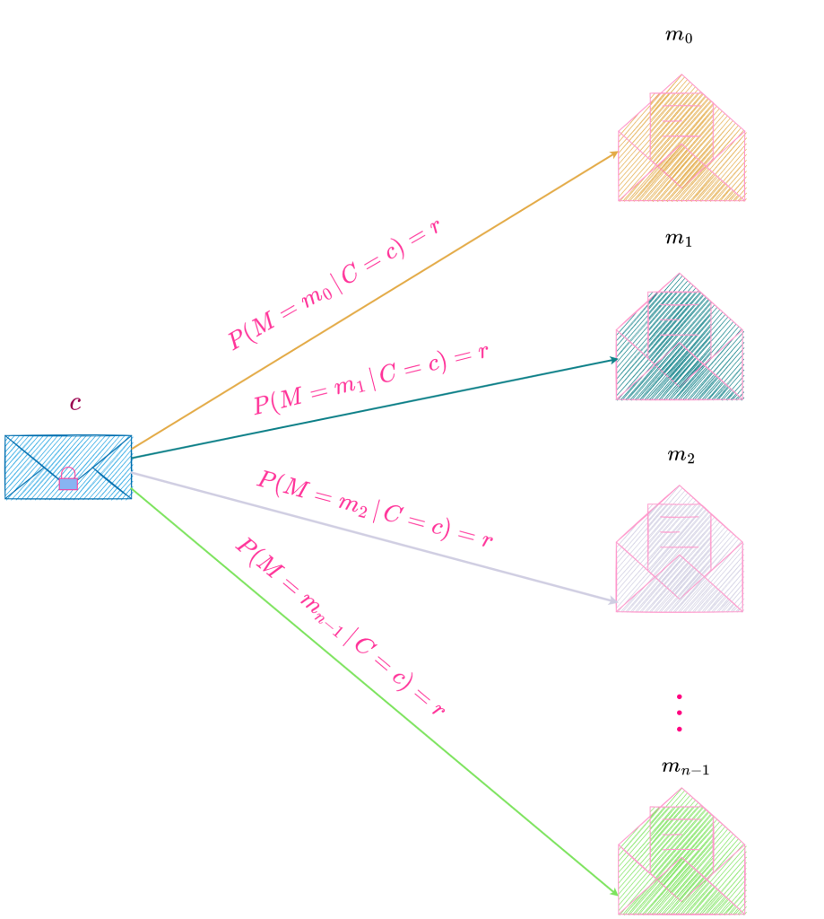
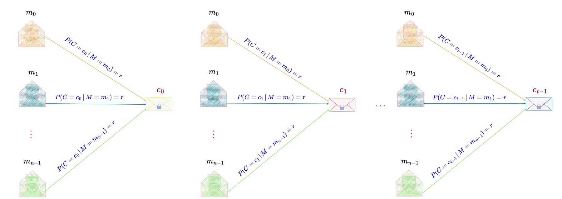
This is illustrated below. Here $r$ is the total probability of all the keys that transform any message $m_i$ to a ciphertext $c$ .

It should be noted that only the total probability of all the keys transforming a message to a ciphertext needs to be equal to that of all the keys transforming any other message to the same ciphertext. The number of keys transforming a message to a ciphertext need not be equal to the number of keys transforming another message to the same ciphertext. Also the keys need not be equally likely i.e., each key can have its own associated probability different from other keys.

A key which enciphers a particular message $m$ into a ciphertext $c$ also deciphers $c$ into the same message $m$ . Hence, the total probability of all keys that transform a message $m_i$ into a given ciphertext $c$ is equal to that of all keys transforming the ciphertext $c$ into the same message $m_i$ , for all $c \text{ and } m_i$ . That is, for every $c \in C$ ,

\begin{align*} P(C = c \,|\,M = m_0) &= P(M = m_0 \,|\,C = c) \,\&\\ P(C = c \,|\,M = m_1) &= P(M = m_1 \,|\,C = c) \,\&\\ &\,\,\,\vdots \\ P(C = c \,|\,M = m_{n-1}) &= P(M = m_{n-1} \,|\,C = c) \\ \end{align*}

We have already shown that,

P(C = c \,|\,M = m_0) = P(C = c \,|\,M = m_1) = \cdots = P(C = c \,|\,M = m_{n-1})

for all $c \in C$ .

Hence,

P(M = m_0 \,|\,C = c) = P(M = m_1 \,|\,C = c) = \cdots = P(M = m_{n-1} \,|\,C = c)

for all $c \in C$ .

This is illustrated below.

This image has an empty alt attribute; its file name is PerfectSecrecyEquation_2-1-919x1024.png

Distribution of Ciphertexts

We will next discuss whether the equation for perfect secrecy constrains the distribution of the ciphertexts in anyway i.e., does it necessitate the ciphertexts to have a particular distribution?

For perfect secrecy,

P(C = c \,|\, M = m) = P(C = c) \neq 0

for every $c \in C \text{ and } m \in M$ .

The following is the necessary and sufficient condition for perfect secrecy enumerated for every $m \text{ and } c$ .

\begin{align*} \small P(C = c_0 \,|\,M = m_0) &= \small P(C = c_0) = r_0 \,\,\& \quad \small P(C = c_1 \,|\,M = m_0) = \small P(C = c_1) = r_1\,\,\& \quad \cdots \quad \small P(C = c_{t-1} \,|\,M = m_0) = \small P(C = c_{t-1}) = r_{t-1}\,\,\&\\ \\ \small P(C = c_0 \,|\,M = m_1) &= \small P(C = c_0) = r_0 \,\,\& \quad \small P(C = c_1 \,|\,M = m_1) = \small P(C = c_1) = r_1\,\,\& \quad \cdots \quad \small P(C = c_{t-1} \,|\,M = m_1) = \small P(C = c_{t-1}) = r_{t-1}\,\,\&\\ \\ &\,\,\,\vdots \quad\quad\quad\quad\quad\quad\quad\quad\quad\quad\quad\quad\quad\quad\quad\quad\,\,\,\,\,\,\vdots \quad\quad\quad\quad\quad\quad\quad\quad\quad\quad\quad\quad\quad\quad\quad\quad\quad\quad\,\,\,\,\,\,\,\,\,\,\,\vdots\\ \\ \small P(C = c_0 \,|\,M = m_{n-1}) &= \small P(C = c_0) = r_0 \quad \quad \small P(C = c_1 \,|\,M = m_{n-1}) = \small P(C = c_1) = r_1\quad \cdots \quad\small P(C = c_{t-1} \,|\,M = m_{n-1}) = \small P(C = c_{t-1}) = r_{t-1} \\ \end{align*}

Here $m$ is the number of messages in the message space and $t$ is the number of ciphertexts in the ciphertext space.

These sets of equations are illustrated below :

We have already seen that a perfect secrecy system satisfies the following equation

P(M = m \,|\, C= c) = P(M = m)

for all $c \text{ and } m$ .

Hence,

\begin{align*} P(M = m_0 \,|\, C= c_0) &= P(M = m_0) \,\& \\ P(M = m_0 \,|\, C= c_1) &= P(M = m_0) \,\& \\ &\,\,\,\vdots \\ P(M = m_0 \,|\, C= c_{t-1}) &= P(M = m_0) \,\& \\ \end{align*}

Therefore,

P(M = m_0 \,|\, C= c_0) = P(M = m_0 \,|\, C= c_1) = \cdots = P(M = m_0 \,|\, C= c_{t-1})

We have already shown above that

\begin{align*} P(C = c_0 \,|\,M = m_0) &= P(M = m_0 \,|\,C = c_0) \,\&\\ P(C = c_1 \,|\,M = m_0) &= P(M = m_0 \,|\,C = c_1) \,\&\\ &\,\,\,\vdots \\ P(C = c_{t-1} \,|\,M = m_0) &= P(M = m_0 \,|\,C = c_{t-1}) \\ \end{align*}

Therefore,

P(C = c_0 \,|\, M= m_0) = P(C = c_1 \,|\, M = m_0) = \cdots = P(C = c_{t-1} \,|\, M= m_0)

The necessary and sufficient condition for perfect secrecy states that,

\begin{align*} P(C = c_0 \,|\,M = m_0) &= P(C = c_0) \,\&\\ P(C = c_1 \,|\,M = m_0) &= P(C = c_1) \,\&\\ &\,\,\,\vdots \\ P(C = c_{t-1} \,|\,M = m_0) &= P(C = c_{t-1}) \\ \end{align*}

Therefore,

P(C = c_0) = P(C = c_1) = \cdots = P(C = c_{t-1})

Hence in a perfectly secure system the ciphertext distribution is uniform.

These relationships are illustrated below:

Relationship between $|K|$ and $|C|$

For perfect secrecy,

P(C = c \,|\, M = m) = P(C = c) \neq 0

for every $c \in C \text{ and } m \in M$ .

We have already shown above that any message in the message space enciphers to any ciphertext in the ciphertext space with equal and non-zero probability i.e., the value of $P(C = c \,|\, M = m)$ is non-zero and the same for any $c \in C \text{ and } m \in M$ .

The following is the enumeration of this result for every $m \in M \text{ and } c \in C$ .

\begin{align*} \small P(C = c_0 \,|\,M = m_0) &= \small P(C = c_0) = r \,\,\& \quad \small P(C = c_1 \,|\,M = m_0) = \small P(C = c_1) = r\,\,\& \quad \cdots \quad \small P(C = c_{t-1} \,|\,M = m_0) = \small P(C = c_{t-1}) = r\,\,\&\\ \\ \small P(C = c_0 \,|\,M = m_1) &= \small P(C = c_0) = r \,\,\& \quad \small P(C = c_1 \,|\,M = m_1) = \small P(C = c_1) = r\,\,\& \quad \cdots \quad \small P(C = c_{t-1} \,|\,M = m_1) = \small P(C = c_{t-1}) = r\,\,\&\\ \\ &\,\,\,\vdots \quad\quad\quad\quad\quad\quad\quad\quad\quad\quad\quad\quad\quad\quad\quad\quad\,\,\,\,\,\,\vdots \quad\quad\quad\quad\quad\quad\quad\quad\quad\quad\quad\quad\quad\quad\quad\quad\quad\quad\,\,\,\,\,\,\,\,\,\,\,\vdots\\ \\ \small P(C = c_0 \,|\,M = m_{n-1}) &= \small P(C = c_0) = r \quad \quad \small P(C = c_1 \,|\,M = m_{n-1}) = \small P(C = c_1) = r\quad \cdots \quad\small P(C = c_{t-1} \,|\,M = m_{n-1}) = \small P(C = c_{t-1}) = r \\ \end{align*}

There are $n$ messages in the message space and $t$ ciphertexts in the ciphertext space.

Below is an illustration of this result i.e., every message in the message space enciphering to every ciphertext in the ciphertext space with equal and non-zero probability, $r$ .

Since $P(C = c \,|\, M = m) = P(C = c) \neq 0$ for any $c \in C \text{ and any } m \in M$ , it must be the case that there is at least one key transforming any $m$ into any of the possible $c\text{'s}$ .

But all the keys transforming a particular message $m$ into different $c\text{'s}$ must be different so that given a message and a key unique encipherment is possible i.e., a key transforms a message into exactly one ciphertext. Therefore, the number of keys is at least equal to the number of ciphertexts, i.e., $|K| \geq |C|$ .

Since a key is first chosen and shared independent of the message that needs to be communicated, it means that a key should be able to encrypt any message in the message space. Hence every key in the key space can encipher any message in the message space.

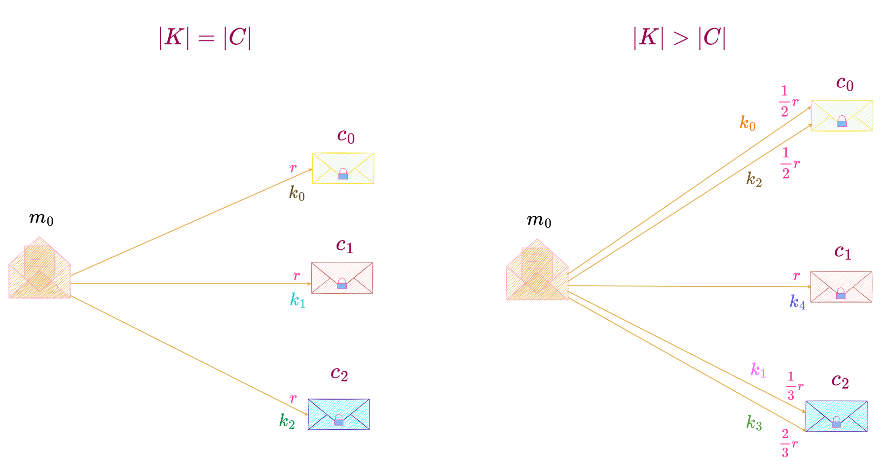
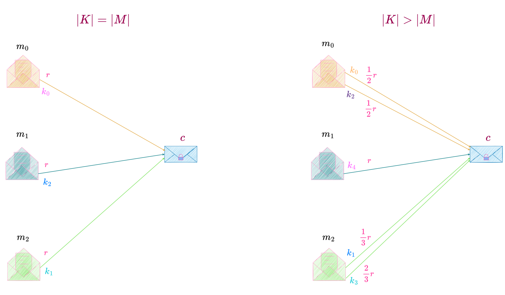
These two cases, $|K| = |C| \text{ and } |K| > |C|$ are illustrated below.

We have already proved that,

P(C = c_0 \,|\, M= m_0) = P(C = c_1 \,|\, M = m_0) = P(C = c_2 \,|\, M= m_0)

Hence, as shown in the illustration above, a particular message in the message space can be transformed into a ciphertext by one or more keys depending on the probability distribution of the keys such that the total probability of all keys that transform the message into a ciphertext is equal to that of all keys that transform the same message to any other ciphertext in the ciphertext space.

We will next consider in some detail examples of perfect secrecy systems with $|K| = |C| \text{ and } |K| > |C|$ .

For the case $|K| = |C|$ , we consider a perfect secrecy system with

$M = \{m_0, m_1, m_2\}, K = \{k_0, k_1, k_2\} \text{ and } C = \{c_0, c_1, c_2\}$ , as shown below.

Since the transformation of a message into a ciphertext corresponds to enciphering with a particular key, the probability of a message resulting in a particular ciphertext equals the sum of probabilities of all keys that transform the message into that ciphertext (since given those keys, a message results in a particular ciphertext with probability 1, i.e., $P(C = c \,|\, M = m, K = k) = 1 \,\forall\, \{k : c = T_k\, m\}$ where $T_k$ is the transformation applied to message $\mathcal{m}$ to produce ciphertext $\mathcal{c}$ . The index $k$ corresponds to the particular key being used.)

Expressed as an equation,

P(C = c \,|\, M = m) = \sum_{k \,\in\, K} P(K = k)\, P(C = c \,|\, M = m, K = k)

In the above example,

\begin{equation*} \begin{split} P(C = c_0 \,|\, M = m_0) & = \sum_{k \,\in\, K} P(K = k)\, P(C = c_0 \,|\, M = m_0, K = k) \\ & = P(K = k_0)\, P(C = c_0 \,|\, M = m_0, K = k_0) \\ & \quad+ P(K = k_1)\, P(C = c_0 \,|\, M = m_0, K = k_1)\\ & \quad + P(K = k_2)\, P(C = c_0 \,|\, M = m_0, K = k_2) \\ & = P(K = k_0) \times 1 + P(K = k_1) \times 0 + P(K = k_2) \times 0 \\ & = P(K = k_0) \end{split} \end{equation*}

Since $P(C = c_0 \,|\, M = m_0) = r, P(K = k_0) =r$ . Similarly, $P(K = k_1) =r \text{ and } P(K = k_2)=r$ .

Therefore,

P(K = k_0) = P(K = k_1)=P(K = k_2)

i.e., when $|K| = |C|$ , the distribution of keys is uniform.

Since $P(C = c_0 \,|\, M= m_0) = P(C = c_1 \,|\, M = m_0) = P(C = c_2 \,|\, M= m_0) = r$ , i.e., the total probability of all keys transforming the message to a particular ciphertext equals that of all keys transforming the same message to any other ciphertext and there is only one key transforming the message to a particular ciphertext, each key has an equal probability, $r$ , of being picked.

For the case $|K| > |C|$ ,

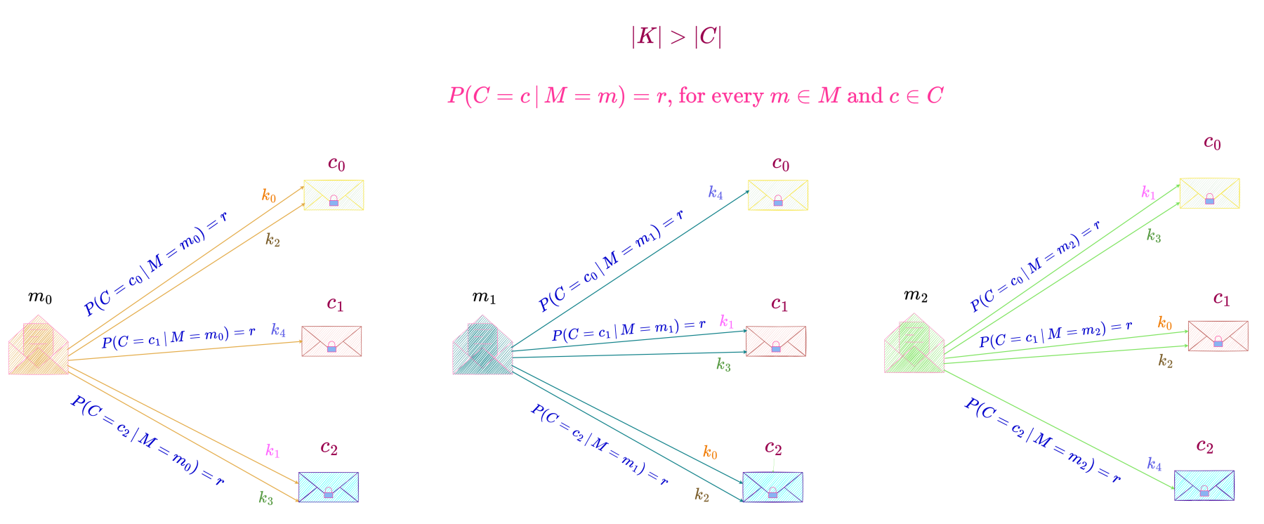
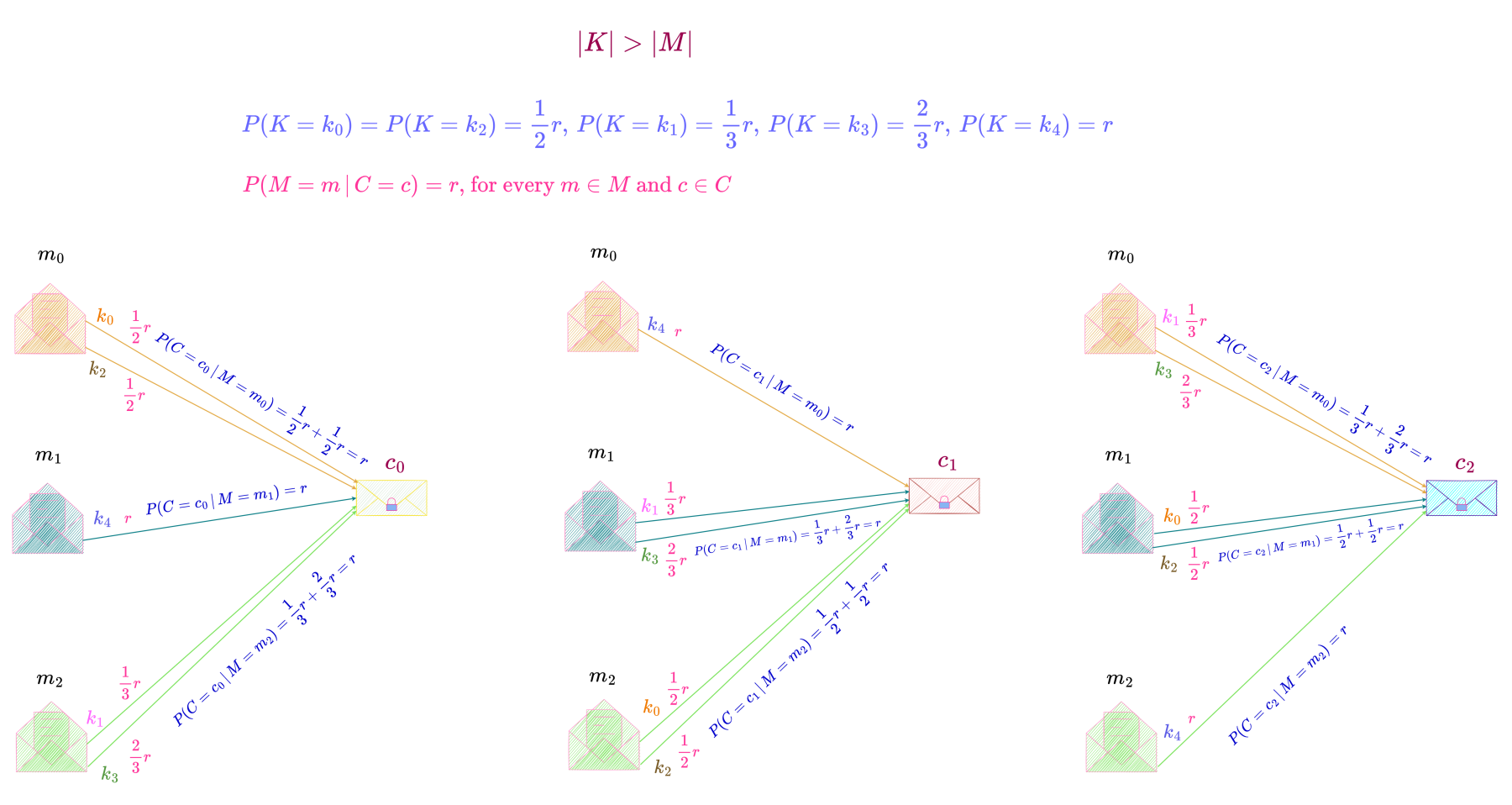
we consider a perfect secrecy system with $M = \{m_0, m_1, m_2\}, K = \{k_0, k_1, k_2, k_3, k_4\} \text{ and } C = \{c_0, c_1, c_2\}$ , as shown below.

For this perfect secrecy system,

\begin{equation*} \begin{split} P(C = c_0 \,|\, M = m_0) & = \sum_{k \,\in\, K} P(K = k)\, P(C = c_0 \,|\, M = m_0, K = k) \\ & = P(K = k_0)\, P(C = c_0 \,|\, M = m_0, K = k_0) \\ & \quad+ P(K = k_1)\, P(C = c_0 \,|\, M = m_0, K = k_1)\\ & \quad + P(K = k_2)\, P(C = c_0 \,|\, M = m_0, K = k_2) \\ & \quad + P(K = k_3)\, P(C = c_0 \,|\, M = m_0, K = k_3) \\ & \quad + P(K = k_4)\, P(C = c_0 \,|\, M = m_0, K = k_4) \\ & = P(K = k_0) \times 1 + P(K = k_1) \times 0 + P(K = k_2) \times 1 + P(K = k_3) \times 0 + P(K = k_4) \times 0\\ & = P(K = k_0) + P(K = k_2) \\ \end{split} \end{equation*}

Since $P(C = c_0 \,|\, M = m_0) = r$ ,

P(K = k_0) + P(K = k_2) = r

Similarly,

\begin{equation*} \begin{split} P(K = k_1) + P(K = k_3) &= r \,\&\\ P(K = k_4) &= r \\ \end{split} \end{equation*}

In this perfect secrecy system, each message can be transformed into a particular ciphertext by either one or two keys. Since a message can be enciphered by every key in the key space, each key has a non-zero probability of being chosen and as can be seen from the above equations, the distribution of keys is non-uniform.

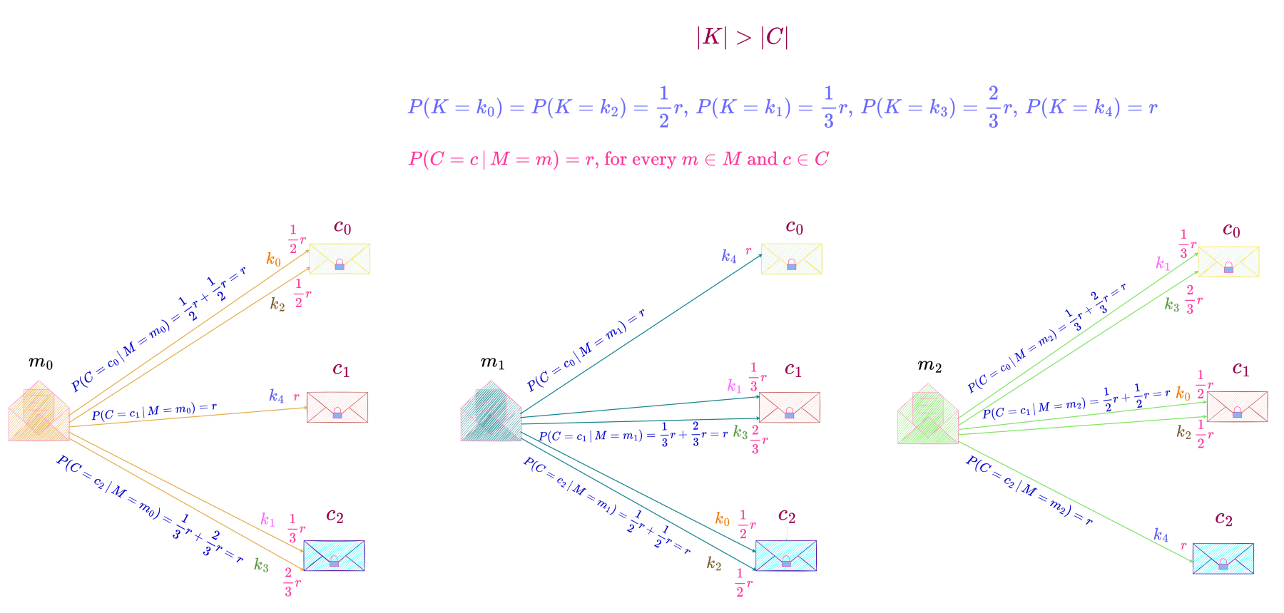
This perfect secrecy system with one possible probability distribution of keys is shown below.

Here,

\begin{align*} P(K = k_0) &= P(K = k_2) = \frac{1}{2}r \\ P(K = k_1) &= \frac{1}{3}r \\ P(K = k_3) &= \frac{2}{3}r \\ P(K = k_4) &= r \\ \end{align*}

Since by the axiom of probability,

P(K = k_0) + P(K = k_1) + P(K = k_2) + P(K = k_3) + P(K = k_4) = 1

it follows that,

\begin{align*} \frac{1}{2}r + \frac{1}{3}r + \frac{1}{2}r + \frac{2}{3}r + r &= 1 \\ 3r &= 1 \\ r &= \frac{1}{3} \\ \end{align*}

Hence,

\begin{align*} P(K = k_0) &= P(K = k_2) = \frac{1}{2}r = \frac{1}{2} \times \frac{1}{3} = \frac{1}{6} \\ P(K = k_1) &= \frac{1}{3}r = \frac{1}{3} \times \frac{1}{3} = \frac{1}{9} \\ P(K = k_3) &= \frac{2}{3}r = \frac{2}{3} \times \frac{1}{3} = \frac{2}{9}\\ P(K = k_4) &= r = \frac{1}{3} \\ \end{align*}

We can see that,

P(C = c \,|\, M = m) = P(K = k_0) + P(K = k_2) = P(K = k_1) + P(K = k_3) = P(K = k_4) = r = \frac{1}{3}

for every $c \in C \text{ and } m \in M$ .

The above equation shows that any message is transformed into any ciphertext by keys $k_0 \text{ and } k_2$ or keys $k_1 \text{ and } k_3$ or key $k_4$ with the same total probability $r = \dfrac{1}{3}$ .

There are more keys than ciphertexts (the key space consists of $5$ keys, while the ciphertext space’s cardinality is $3$ ) since a message is transformed into a ciphertext by one or two keys, such that $P(C = c \,|\, M = m) = r$ for every $c \in C \text{ and } m \in M$ and all the keys transforming a particular message $m$ into different $c \text{'s}$ must be different.

Hence, $|K| \geq |C|$ .

Relationship between $|K|$ and $|M|$

We have already shown that any message in the message space enciphers to any ciphertext in the ciphertext space with equal and non-zero probability i.e., the value of $P(C = c \,|\, M = m)$ is non-zero and the same for any $c \in C \text{ and } m \in M$ .

Below is an illustration of this result i.e., every message in the message space enciphering to every ciphertext in the ciphertext space with equal and non-zero probability, $r$ .

But all the keys transforming different messages into a particular ciphertext $c$ must be different so that given a ciphertext and key unique decipherment is possible. Therefore, the number of keys is at least equal to the number of messages, i.e., $|K| \geq |M|$ .

It should also be noted that since a key is first chosen and shared independent of the message that needs to be communicated, it means that a key should be able to encrypt any message in the message space. Hence every key in the key space can encipher any message in the message space.

These two cases, $|K| = |M| \text{ and } |K| > |M|$ are illustrated below.

Let us next consider two examples of perfect secrecy systems one with $|K| = |M| \text{ and other with } |K| > |M|$ .

For the case $|K| = |M|$ , we consider a perfect secrecy system with

$M = \{m_0, m_1, m_2\}, K = \{k_0, k_1, k_2\} \text{ and } C = \{c_0, c_1, c_2\}$ , as shown below.

As we have already shown in the case where $|K| = |C|$ ,

\begin{equation*} \begin{split} P(C = c_0 \,|\, M = m_0) & = \sum_{k \,\in\, K} P(K = k)\, P(C = c_0 \,|\, M = m_0, K = k) \\ & = P(K = k_0) \end{split} \end{equation*}

Similarly,

P(C = c_0 \,|\, M = m_1) = P(K = k_1)

and

P(C = c_0 \,|\, M = m_2) = P(K = k_2)

Since

P(C = c_0 \,|\, M = m_0) = P(C = c_0 \,|\, M = m_1) = P(C = c_0 \,|\, M = m_2)

it follows that,

P(K = k_0) = P(K = k_1)=P(K = k_2)

i.e., when $|K| = |M|$ , the distribution of keys is uniform.

For the case $|K| > |M|$ ,

we consider a perfect secrecy system with $M = \{m_0, m_1, m_2\}, K = \{k_0, k_1, k_2, k_3, k_4\} \text{ and } C = \{c_0, c_1, c_2\}$ , as shown below.

As we have already shown in the case where $|K| > |C|$ ,

P(C = c \,|\, M = m) = P(K = k_0) + P(K = k_2) = P(K = k_1) + P(K = k_3) = P(K = k_4) = r = \frac{1}{3}

for every $c \in C \text{ and } m \in M$ .

In this perfect secrecy system there are more keys than messages (the key space consists of $5$ keys, while the message space’s cardinality is $3$ ) because a message is transformed into a ciphertext by one or two keys, such that $P(C = c \,|\, M = m) = r$ for every $c \in C \text{ and } m \in M$ and all the keys transforming different messages $m$ into a particular ciphertext $c$ must be different so that given a ciphertext and key unique decipherment is possible.

Hence, $|K| \geq |M|$ .

Relationship between $|C|$ and $|M|$

Since any key in the key space enciphers every message in the message space to a different ciphertext such that given the ciphertext and key, unique decipherment is possible, there must be at least as many ciphertexts as there are messages i.e.,

|C| \geq |M|

We illustrate the two cases, namely, $|C| = |M| \text{ and } |C| > |M|$ below.

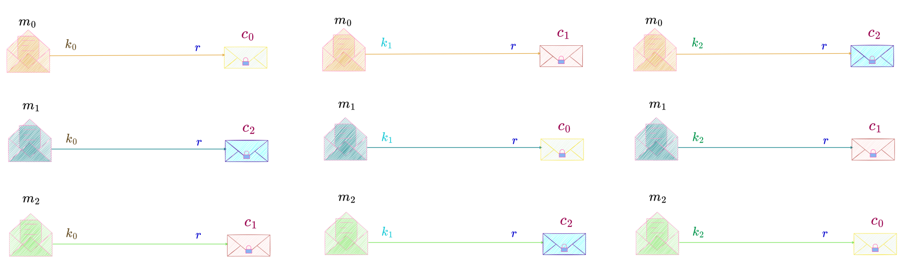
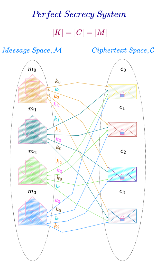
Below is the illustration of a perfect secrecy system with $|C| = |M|$ , where the message space consists of $3$ messages, the key space consists of $3$ keys and the ciphertext space also consists of $3$ ciphertexts. The keys are drawn from a uniform distribution and the probability of choosing a key is $\dfrac{1}{3}$ , i.e., $r = \dfrac{1}{3}$ .

We can see that for any key in the key space there is a one-to-one correspondence between all the messages in the message space and all the ciphertexts in the ciphertext space.

Next let us explore the case when $|C| > |M|$ .

From the two illustrations shown below depicting the cases $|K| = |M| \text{ and } |K| > |M|$ , we can see that the entire key space is exhausted by all the messages that transform to a particular ciphertext i.e., every message in the message space transforms to a particular ciphertext through some permutation of the entire key space.

From the illustration on the left, where $|K| = |M|$ , we can see that some permutation of the entire key space i.e., $K = \{k_0, k_1, k_2\}$ transforms the message space i.e., $M = \{m_0, m_1, m_2\}$ into a particular ciphertext, $c$ .

Similarly, in the illustration on the right, where $|K| > |M|$ , some permutation of the entire key space i.e., $K = \{k_0, k_1, k_2, k_3, k_4\}$ transforms the message space i.e., $M = \{m_0, m_1, m_2\}$ into a particular ciphertext, $c$ .

However, in some cases when $|K| > |M|$ , depending on the probability distribution of the keys, only a subset of the key space is exhausted (used) when the message space is transformed to a particular ciphertext as explained below.

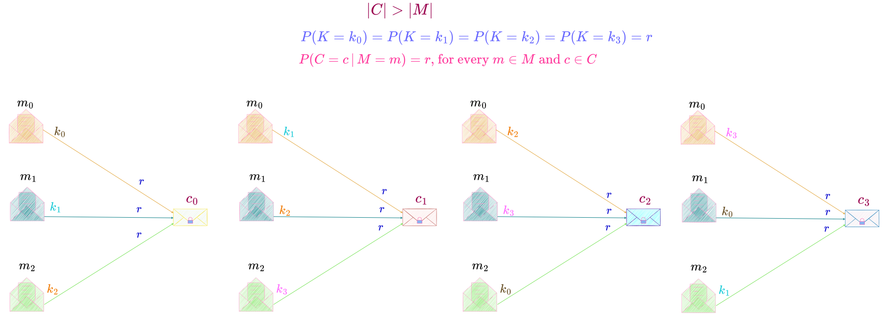
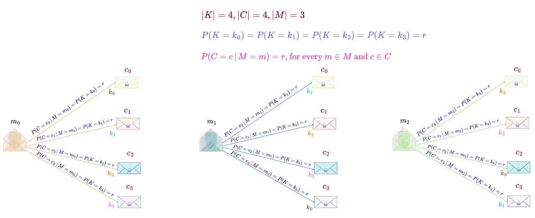
Consider a perfect secrecy system where the key space consists of $4$ keys, all equally likely and the message space consists of only $3$ messages.

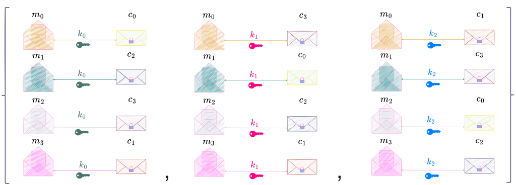
In a perfect secrecy system, the probability that a message transforms to a particular ciphertext equals that of the message transforming to any other ciphertext in the ciphertext space. Since in this particular perfect secrecy system every key in the key space has an equal probability, $r$ , of being picked, and every key in the key space can encipher any message in the message space, each key in the key space transforms a particular message into a unique ciphertext so that the probability of the message transforming to any ciphertext in the ciphertext space is the same and equals $r$ . Hence, each of the $4$ keys encipher a particular message into $4$ different ciphertexts as shown below. Since each of the $3$ messages in the message space are transformed into $4$ different ciphertexts by $4$ equally likely keys, in this case, $|C| > |M|$ .

Since there are only $3$ messages and each key is equally likely, there is only one unique key that transforms each of those messages into a particular ciphertext. Hence here only $3$ out of the $4$ keys are used to transform the message space into a particular ciphertext i.e., the entire key space is not used to transform the message space into a ciphertext. In the example shown above only keys $k_0, k_1 \text{ and } k_2$ are used to transform the $3$ messages $m_0, m_1 \text{ and } m_2$ into ciphertext $c_0$ .

Therefore, for every key in the key space, there is a one-to-one correspondence between all messages in the message space and some of the ciphertexts in the ciphertext space.

This case of $|C| > |M|$ is illustrated below. Since the keys are drawn from a uniform distribution and there are four keys, $r = \dfrac{1}{4}$ .

We can see from the above illustration that every message is enciphered by all the four keys (since a key should be able to encipher any message in the message space), but every ciphertext is not deciphered by all the keys (in fact only $3$ keys decipher each ciphertext). So for any fixed key there is a one-to-one correspondence between all the messages in the message space, and some of the ciphertexts in the ciphertext space.

For example, for the key $k_0$ , there is a one-to-one correspondence between the messages $m_0, m_1 \text{ and } m_2$ and the ciphertexts $c_0, c_3 \text{ and } c_2$ i.e., a one-to-one correspondence between all the $3$ messages in the message space and $3$ out of the $4$ ciphertexts in the ciphertext space. This is a consequence of $|K| > |M|$ and each key being equally likely i.e., the key space having a uniform distribution (and also the total probability of each message transforming to a particular ciphertext requiring to equal that of every other message transforming to the same ciphertext).

It should be noted that though all keys don’t decipher a particular ciphertext, a ciphertext still deciphers to every message in the message space with equal probability and also every message in the message space also enciphers to every ciphertext in the ciphertext space with equal probability. Hence perfect secrecy is still maintained.

So far we have proved that,

\begin{equation*} \begin{split} |K| & \geq |C| \\ |K| & \geq |M| \text{ and} \\ |C| & \geq |M| \\ \end{split} \end{equation*}

It follows from the above inequalities that,

|K| \geq |C| \geq |M|

As an aside, though we don’t need $|K| \geq |M|$ to prove the above relationship, we needed it to prove $|C| \geq |M|$ .

Various kinds of Perfect Secrecy Systems

Perfect Secrecy System with $|K| > |C| > |M|$

By axiom of probability,

\begin{equation*} \begin{split} P(C = c_0 \,|\, M = m_0) + P(C = c_1 \,|\, M = m_0) + P(C = c_2 \,|\, M = m_0)&= 1 \\ r + r + r &= 1\\ 3r &= 1 \\ r &= \frac{1}{3}\\ \end{split} \end{equation*}

Also,

\begin{equation*} \begin{split} P(C = c) &= \sum_{m \,\in\, M} P(M = m)\, P(C = c \,|\, M = m) \\ &= \sum_{m \,\in\, M} P(M = m) \times r \\ &= r \sum_{m \,\in\, M} P(M = m) \\ &= r \\ \end{split} \end{equation*}

for every $c \in C$ , since $P(C = c \,|\, M = m) = r$ for every $c \in C \text{ and } m \in M$ and by axiom of probability, $\displaystyle \sum_{m \,\in\, M} P(M = m) = 1$ .

Therefore,

P(C = c \,|\, M = m) = P(C = c) = \frac{1}{3}

for all $c \in C \text{ and } m \in M$ .

Also,

\begin{equation*} \begin{split} P(C = c_0 \,|\, M = m_0) & = \sum_{k \,\in\, K} P(K = k)\, P(C = c_0 \,|\, M = m_0, K = k) \\ & = P(K = k_0) \end{split} \end{equation*}

Similarly,

P(C = c_1 \,|\, M = m_0) = P(K = k_1)

and

P(C = c_2 \,|\, M = m_0) = P(K = k_2) + P(K = k_3)

Therefore,

P(K = k_0) = P(K = k_1) = r = \frac{1}{3}

and

P(K = k_2) = P(K = k_3) = \frac{1}{2}r = \frac{1}{6}

In this perfect secrecy system, each message is transformed to a particular ciphertext by one or two keys.

Also, for every key in the key space there is a one-to-one correspondence between all the messages in the message space and some of the ciphertexts in the ciphertext space. For example, for key $k_0$ , there is a one-to-one correspondence between messages $m_0 \text{ and } m_1$ and ciphertexts $c_0 \text{ and } c_1$ .

The distribution of keys is non-uniform.

Perfect Secrecy System with $|K| > |C| = |M|$

By axiom of probability,

\begin{equation*} \begin{split} P(C = c_0 \,|\, M = m_0) + P(C = c_1 \,|\, M = m_0) &= 1 \\ \frac{3}{2}r + \frac{3}{2}r &= 1\\ 3r &= 1 \\ r &= \frac{1}{3}\\ \end{split} \end{equation*}

Also,

\begin{equation*} \begin{split} P(C = c) &= \sum_{m \,\in\, M} P(M = m)\, P(C = c \,|\, M = m) \\ &= \sum_{m \,\in\, M} P(M = m) \times \frac{3}{2}r \\ &= \frac{3}{2}r \sum_{m \,\in\, M} P(M = m) \\ &= \frac{3}{2}r \\ \end{split} \end{equation*}

for every $c \in C$ , since $P(C = c \,|\, M = m) = \dfrac{3}{2}r$ for every $c \in C \text{ and } m \in M$ and by axiom of probability, $\displaystyle \sum_{m \,\in\, M} P(M = m) = 1$ .

Therefore,

P(C = c \,|\, M = m) = P(C = c) = \frac{3}{2}r =\frac{1}{2}

for all $c \in C \text{ and } m \in M$ .

Also,

\begin{equation*} \begin{split} P(C = c_0 \,|\, M = m_0) & = \sum_{k \,\in\, K} P(K = k)\, P(C = c_0 \,|\, M = m_0, K = k) \\ & = P(K = k_0) + P(K = k_2) \\ \end{split} \end{equation*}

Similarly,

P(C = c_1 \,|\, M = m_0) = P(K = k_1) + P(K = k_3)

As can be seen from the above illustration,

P(K = k_0) = P(K = k_1) = r = \frac{1}{3}

and

P(K = k_2) = P(K = k_3) = \frac{1}{2}r = \frac{1}{6}

In this perfect secrecy system, each message is transformed to a particular ciphertext by exactly two keys.

Also, for every key in the key space there is a one-to-one correspondence between all the messages in the message space and all the ciphertexts in the ciphertext space.

The distribution of keys is non-uniform.

Perfect Secrecy System with $|K| = |C| > |M|$

By axiom of probability,

\begin{equation*} \begin{split} P(C = c_0 \,|\, M = m_0) + P(C = c_1 \,|\, M = m_0) + P(C = c_2 \,|\, M = m_0) + P(C = c_3 \,|\, M = m_0)&= 1 \\ r + r + r + r &= 1\\ 4r &= 1 \\ r &= \frac{1}{4}\\ \end{split} \end{equation*}

Also,

\begin{equation*} \begin{split} P(C = c) &= \sum_{m \,\in\, M} P(M = m)\, P(C = c \,|\, M = m) \\ &= \sum_{m \,\in\, M} P(M = m) \times r \\ &= r \sum_{m \,\in\, M} P(M = m) \\ &= r \\ \end{split} \end{equation*}

for every $c \in C$ , since $P(C = c \,|\, M = m) = r$ for every $c \in C \text{ and } m \in M$ and by axiom of probability, $\displaystyle \sum_{m \,\in\, M} P(M = m) = 1$ .

Therefore,

P(C = c \,|\, M = m) = P(C = c) = \frac{1}{4}

for all $c \in C \text{ and } m \in M$ .

Also,

\begin{equation*} \begin{split} P(C = c_0 \,|\, M = m_0) & = \sum_{k \,\in\, K} P(K = k)\, P(C = c_0 \,|\, M = m_0, K = k) \\ & = P(K = k_0) \end{split} \end{equation*}

Similarly,

\begin{equation*} \begin{split} P(C = c_1 \,|\, M = m_0) &= P(K = k_1), \\ P(C = c_2 \,|\, M = m_0) &= P(K = k_2)\& \\ P(C = c_3 \,|\, M = m_0)&= P(K = k_3) \\ \end{split} \end{equation*}

Therefore,

P(K = k_0) = P(K = k_1) = P(K = k_2) = P(K = k_3) = r = \frac{1}{4}

In this perfect secrecy system, each message is transformed to a particular ciphertext by exactly one key. Hence, the distribution of keys is uniform.

Also, for every key in the key space there is a one-to-one correspondence between all the messages in the message space and some of the ciphertexts in the ciphertext space. For example, for key $k_0$ , there is a one-to-one correspondence between messages $m_0, m_1 \text{ and } m_2$ and ciphertexts $c_0, c_3 \text{ and } c_2$ .

Perfect Secrecy System with $|K| = |C| = |M|$

By axiom of probability,

\begin{equation*} \begin{split} P(C = c_0 \,|\, M = m_0) + P(C = c_1 \,|\, M = m_0) + P(C = c_2 \,|\, M = m_0) + P(C = c_3 \,|\, M = m_0)&= 1 \\ r + r + r + r &= 1\\ 4r &= 1 \\ r &= \frac{1}{4}\\ \end{split} \end{equation*}

Also,

\begin{equation*} \begin{split} P(C = c) &= \sum_{m \,\in\, M} P(M = m)\, P(C = c \,|\, M = m) \\ &= \sum_{m \,\in\, M} P(M = m) \times r \\ &= r \sum_{m \,\in\, M} P(M = m) \\ &= r \\ \end{split} \end{equation*}

for every $c \in C$ , since $P(C = c \,|\, M = m) = r$ for every $c \in C \text{ and } m \in M$ and by axiom of probability, $\displaystyle \sum_{m \,\in\, M} P(M = m) = 1$ .

Therefore,

P(C = c \,|\, M = m) = P(C = c) = \frac{1}{4}

for all $c \in C \text{ and } m \in M$ .

Also,

\begin{equation*} \begin{split} P(C = c_0 \,|\, M = m_0) & = \sum_{k \,\in\, K} P(K = k)\, P(C = c_0 \,|\, M = m_0, K = k) \\ & = P(K = k_0) \end{split} \end{equation*}

Similarly,

\begin{equation*} \begin{split} P(C = c_1 \,|\, M = m_0) &= P(K = k_1), \\ P(C = c_2 \,|\, M = m_0) &= P(K = k_2)\& \\ P(C = c_3 \,|\, M = m_0)&= P(K = k_3) \\ \end{split} \end{equation*}

Therefore,

P(K = k_0) = P(K = k_1) = P(K = k_2) = P(K = k_3) = r = \frac{1}{4}

In this perfect secrecy system, each message is transformed to a particular ciphertext by exactly one key. Hence, the distribution of keys is uniform.

Also, for every key in the key space there is a one-to-one correspondence between all the messages in the message space and all the ciphertexts in the ciphertext space. For example, for key $k_0$ , there is a one-to-one correspondence between messages $m_0, m_1, m_2 \text{ and } m_3$ and ciphertexts $c_0, c_3, c_2 \text{ and } c_1$ .

Perfect secrecy systems in which the number of keys, the number of messages and the number of ciphertexts are all equal are characterized by the following properties :

Every message in the message space is transformed to a particular ciphertext in the ciphertext space by exactly one key.
All the keys in the key space are equally likely.

Hence, from an implementation perspective the simplest (or easiest) possible perfect secrecy system to build is one in which the number of keys, the number of messages and the number of ciphertexts are all equal, i.e.,

|K| = |C| = |M|

Reusing keys makes a Perfect Secrecy System Insecure

Since a perfect secrecy system transforms a message into a ciphertext in a deterministic way i.e., the same message will always generate the same ciphertext for the same key, as we have already discussed, reusing the key to encipher more than one message will make the prefect secrecy system insecure.

The following example shows how a perfect secrecy system can become insecure if the same key is used to encipher more than one message.

Suppose Maria decides to lives between Paris and Milan during the next $100$ days. She will spend $80\%$ of her time in Paris and the remaining $20\%$ in Milan i.e., $80$ days in Paris and $20$ days in Milan. Also, in every $10$ days period she will spend between $1 \text{ to } 3$ days in Milan and the remaining days in Paris. She would like to communicate her location to Bob every single day in secrecy so that no one else knows her whereabouts. They use a simple perfect secrecy system as detailed below.

Let us consider two scenarios, namely, one in which Maria shares a key with Bob only once and then reuses the same key to encipher her location and send it to Bob every time she communicates her location to him. In the other scenario, every time Maria wishes to communicate her location to Bob she picks a key at random from the key space and then encrypts the message (location) using that key. Let us analyze the security of the perfect secrecy system in both these scenarios.

In the first scenario, Maria meets Bob before leaving for Paris and shares key $k_1$ with him. Over the next $100$ days she will use this key to encrypt her communication with Bob.

Following table shows her location for the first ten days, together with the ciphertext she sent to Bob each day to communicate her location to him encrypted using the shared key $k_1$ .

Suppose an eavesdropper intercepts the communication between Maria and Bob and observes the ciphertexts. He will see that $7$ days the location was encrypted to $c_1$ and $3$ days to $c_0$ . Suppose he is aware of the probability distribution of the message space i.e., Maria spending majority of the time in Paris, then observing that $c_1$ occurs more frequently than $c_0$ he will rightly deduce that ciphertext $c_1$ is the encryption of Paris and $c_0$ of Milan. Hence without even knowing the encryption key, he will be able to decipher the message and hence know where Maria will be each day by intercepting the ciphertext alone, thereby making the secrecy system useless.

Let us now consider an alternate scenario. Maria meets Bob each day and shares with him a key which she picks at random. Next day using this key, she encrypts her location and sends it to Bob and Bob meets her at that location.

Following table shows her location for the first ten days, together with the ciphertext she sent to Bob each day to communicate her location to him encrypted using the shared key $k_0 \text{ or } k_1$ which she picked at random with equal probability.

Suppose an eavesdropper observes the ciphertexts that Maria sends to Bob. He sees that on $6$ days $c_1$ was sent and $4$ days $c_0$ was sent. Since he is aware that Maria spends majority of her days in Paris, he assumes $c_1$ to be the encryption of Paris and $c_0$ Milan. Now suppose he decrypts under this assumption. Looking at the table, we can see that he will be right on days $1, 4, 7, 9 \text{ and } 10$ and wrong on days $2, 3, 5, 6 \text{ and } 8$ i.e., he is right on $5$ days and wrong on $5$ days, which is no better than making a random guess each day on Maria’s location. Even if he assumes the contrary, i.e., $c_1$ as the encryption of Milan and $c_0$ that of Paris, he will still be right only $50\%$ of the time. Hence, when the key is not reused the ciphertext reveals no information about the message.

Summary

Before proceeding further, we will summarize our discussion so far.

Necessary and Sufficient Condition for Perfect Secrecy

A necessary and sufficient condition for perfect secrecy is that

P(C = c \,|\,M = m) = P(C = c)

for all $m \text{ and } c$ ; i.e., the message and the ciphertext distributions are independent of each other.

Consequences of Perfect Secrecy

The necessary and sufficient condition for perfect secrecy i.e., the message and the ciphertext distribution being independent of one another, gives rise to the following consequences :

The distribution of ciphertexts is uniform.
Any message in the message space enciphers to any ciphertext in the ciphertext space with equal and non-zero probability i.e., the value of $P(C = c \,|\, M = m)$ is non-zero and the same for any $c \in C \text{ and } m \in M$ .
The size (or cardinality) of the key space, $K$ , must at least equal that of the ciphertext space, $C$ , i.e., $|K| \geq |C|$ .
The cardinality of the key space must at least equal that of the message space i.e., $|K| \geq |M|$ .
The cardinality of the ciphertext space must at least equal that of the message space i.e., $|C| \geq |M|$ .
From $3 \text{ and } 5$ , we can see that $|K| \geq |C| \geq |M|$ .

Practical Implementation of a Perfect Secrecy System

Now that we have discussed in depth the various criteria for secrecy systems to be perfectly secure, let us next proceed to an implementation of a perfect secrecy system. One example of a practical perfect secrecy system is a one-time pad which we will cover in depth in the following section.

To be continued…

cryptography mathematics

Does security against message recovery imply semantic security?

Post author By premmi
Post date November 9, 2023

authored by Premmi and Beguène

We will answer this question using the proof by counterexample method.

We will construct a cipher that is secure against message recovery but is not semantically secure.

Let $\mathcal{E} = (E, D)$ be a semantically secure cipher defined over $(\mathcal{K, M, C})$ , where $\mathcal{K} \subseteq \mathcal{M}$ and $\mathcal{M} = \mathcal{C} = \{0, 1\}^L$ . We will construct a cipher $\tilde{\mathcal{E}} = (\tilde{E}, \tilde{D})$ derived from $\mathcal{E}$ such that $\tilde{\mathcal{E}}$ is secure against message recovery but is not semantically secure.

The encryption and decryption algorithms, $\tilde{E} \text{ and } \tilde{D}$ , respectively, of the cipher $\tilde{\mathcal{E}}$ are defined as follows:

\tilde{E}(k,m) := \text{parity}(m)\parallel E(k, m) \,\,\text{ and }\,\, \tilde{D}(k,c) := D(k, c[1..L-1])

For a bit string $s$ , $\text{parity}(s)$ is $1$ if the number of $1\text{'s}$ in $s$ is odd, and $0$ otherwise.

Let us now prove that $\tilde{\mathcal{E}}$ is secure against message recovery but is not semantically secure.

We will first prove that $\tilde{\mathcal{E}}$ is not semantically secure.

In the semantic security attack game, suppose an efficient adversary picks two messages, say, $m_0 \text{ and } m_1$ such that $\text{parity}(m_0) = 0 \text{ and } \text{parity}(m_1) = 1$ and sends both these messages to the challenger. The challenger picks one of these messages uniformly at random and encrypts the chosen message using the encryption algorithm $\tilde{E}$ of cipher $\tilde{\mathcal{E}}$ and sends the resulting ciphertext to the adversary. Depending on whether the first bit of the ciphertext is $0 \text{ or } 1$ , the adversary will know whether message $m_0 \text{ or } m_1$ was encrypted, thereby always winning the game i.e., the adversary’s semantic security advantage in attacking $\tilde{\mathcal{E}}$ through the challenger will be $1$ i.e., non-negligible. Hence, we have proved that $\tilde{\mathcal{E}}$ is not semantically secure.

Next we will prove that $\tilde{\mathcal{E}}$ is secure against message recovery.

In the message recovery attack game, the challenger picks a message at random from a uniform distribution of messages in the message space. The challenger encrypts this message using the encryption algorithm $\tilde{E}$ of cipher $\tilde{\mathcal{E}}$ and sends the resulting ciphertext $\tilde{c}$ to the efficient adversary. The efficient adversary tries to recover the message whose encryption resulted in $\tilde{c}$ . In order to recover the message, the adversary tries to decrypt the ciphertext, $\tilde{c}$ , whose first bit is the parity of the message that was encrypted and the remaining bits are the bits of the ciphertext $c$ which is the output of the encryption algorithm $E$ of cipher $\mathcal{E}$ .

Suppose it were possible for an efficient adversary to use the parity of a message to recover with non-negligible probability the message from a given ciphertext. Let us call this adversary message recovery using parity adversary. Then in a semantic security attack game, the efficient adversary would pick two messages of the same parity, say $0$ and send these to its challenger. The challenger would pick uniformly at random one of these two messages, encrypt it using cipher $\mathcal{E}$ and send the resulting ciphertext to the adversary. Since the parity of the message is known to be $0$ , this adversary would use the message recovery using parity adversary to recover with non-negligible probability the message from the given ciphertext and hence detect with non-negligible probability which one of two possible messages was encrypted. This implies that $\mathcal{E}$ would not be semantically secure. But since $\mathcal{E}$ is semantically secure such an attack using the parity of the message is not possible.

Hence, in the ciphertext $\tilde{c}$ output by the encryption algorithm $\tilde{E}$ of cipher $\tilde{\mathcal{E}}$ , the first bit of $\tilde{c}$ which is the parity of the message that was encrypted does not help in successfully doing a semantic security attack on the remaining bits of $\tilde{c}$ which are the bits of the ciphertext $c$ output by the encryption algorithm $E$ of cipher $\mathcal{E}$ . We have already proved that if $\mathcal{E}$ is semantically secure, it is also message recovery secure. Since $c = \tilde{c}[1..L-1]$ is the ciphertext output by the encryption algorithm $E$ of cipher $\mathcal{E}$ , and $\mathcal{E}$ is message recovery secure, the message cannot be recovered from the ciphertext $c$ with non-negligible probability. Since $\tilde{c}$ is the parity of the encrypted message concatenated with $c$ and we have shown that $c$ is message recovery secure even when the parity of the encrypted message is known, $\tilde{c}$ is message recovery secure. Hence, $\tilde{\mathcal{E}}$ is message recovery secure.

We have proved that $\tilde{\mathcal{E}}$ is secure against message recovery but is not semantically secure.

Therefore, we can conclude that security against message recovery does not imply semantic security.

cryptography mathematics

Security Proof : Semantic Security implies Message Recovery Security

Post author By premmi
Post date November 8, 2023

authored by Premmi and Beguène

A cipher that is semantically secure is also secure against message recovery.

Prerequisites : Probability Primer, Attack Games In Cryptography, Proof Techniques in Cryptography

Theorem

Let $\mathcal{E} = (E, D)$ be a cipher defined over $(\mathcal{K, M, C})$ . If $\mathcal{E}$ is semantically secure then $\mathcal{E}$ is secure against message recovery.

Intuitively, this theorem means that if an efficient adversary (running time poly-bounded with over-whelming probability) is given a ciphertext which is the encryption of one of the two messages chosen by it and this adversary cannot detect from the given ciphertext which message was encrypted, then it implies that it cannot also recover the message from the ciphertext. This is because had the adversary been able to recover the message from the ciphertext, then it would have known which one of the two messages was encrypted by the cipher $\mathcal{E}$ and hence would have correctly detected the message that the given ciphertext was an encryption of.

In order to prove this theorem, we need to find a way to relate the semantic security of cipher $\mathcal{E}$ to its security against message recovery. We will establish this relationship through a game wherein an efficient semantic security adversary tries to break the semantic security of cipher $\mathcal{E}$ by using an efficient message recovery adversary.

A message recovery adversary when given a ciphertext tries to recover the message from the ciphertext. A semantic security adversary, on the other hand, when given a ciphertext, which is the encryption of one of two possible messages of its choosing, tries to detect which message was encrypted. Therefore, a semantic security adversary, when given a ciphertext, can use a message recovery adversary to recover the message from the ciphertext and hence detect which one of the two possible messages was encrypted to result in the given ciphertext.

It should be noted that the only purpose of the game is to establish a relationship between the two notions of security; had their relationship been already known then we don’t need this game as we can the prove the theorem using this relationship.

How secure a cipher is against a particular notion of security attack is quantified as the advantage that an adversary has over a challenger whose output the adversary uses to attack the cipher, in a game played between them. Since the advantage of the adversary over the challenger is a measure of the difference in probabilities between the adversary winning the game and the challenger winning the game, hence, the higher the advantage of the adversary over the challenger, the lesser the security of the cipher for the particular notion of security under attack.

Therefore, in order to relate the semantic security of the given cipher $\mathcal{E}$ to its security against message recovery, we have to formulate a relationship between the advantage that an efficient semantic security adversary has over its challenger and the advantage that an efficient message recovery adversary has over its challenger. We establish this relationship through a game as described below.

It should be noted that efficient adversary / interface means its running time is poly-bounded with overwhelming probability or equivalently, unbounded with at most negligible probability..

Also SS denotes “Semantic Security” and MR denotes “Message Recovery”.

The game is played as follows :

The efficient SS Adversary $\mathcal{B}$ picks any two messages of its choice, namely, $m_0 \text{ and } m_1$ , from the message space $\mathcal{M}$ and sends them to its SS Challenger, $\mathcal{C_B}$ . It should be noted that $m_0 \text{ and } m_1$ are two different messages i.e., $m_0 \neq m_1$ .
The SS Challenger, $\mathcal{C_B}$ chooses either $m_0 \text{ or } m_1$ uniformly at random, encrypts it using cipher $\mathcal{E}$ and sends the ciphertext $c$ to $\mathcal{B}$ . The challenger, $\mathcal{C_B}$ , chooses the message to encrypt uniformly at random to ensure that the adversary $\mathcal{B}$ wins the game only by correctly detecting from the given ciphertext which one of the two messages was encrypted by the challenger and not by exploiting the bias (or preference) of $\mathcal{C_B}$ in picking one message over the other.
$\mathcal{B}$ forwards $c$ to its MR Adversary $\mathcal{A}$ through its interface, $\mathcal{C_A}$ , which acts as MR Challenger to $\mathcal{A}$ .
$\mathcal{A}$ tries to recover the message from the given ciphertext $c$ and outputs a message $\hat{m} \in \{m_0, m_1\}$ which it sends to its MR Challenger i.e., $\mathcal{B} \text{'s}$ interface $\mathcal{C_A}$ . It should be noted that since $c$ is an encryption of either $m_0 \text{ or } m_1$ , in the message recovery game the message space consists of just these two messages.
The adversary $\mathcal{B}$ outputs $\hat{b} = 1$ when $\hat{m} = m_1$ and outputs $\hat{b} = 0$ when $\hat{m} = m_0$ . $\mathcal{B}$ sends $\hat{b}$ to its SS Challenger, $\mathcal{C_B}$ .

For $b = 0, 1$ , efficient MR Adversary, $\mathcal{A}$ , wins the game against its MR Challenger, $\mathcal{C_A}$ , if $c$ is the encryption of $m_b$ and it outputs $\hat{m} = m_b$ , otherwise it loses and consequently, its MR Challenger, $\mathcal{C_A}$ , wins the game.

By definition,

\begin{equation*} \begin{split} \text{MR}\bold{adv}[\mathcal{A, C_A}] &= \big|P(\hat{m} = m_1 \,|\, c \text{ is encryption of } m_0) -P(\hat{m} = m_1 \,|\, c \text{ is encryption of } m_1)\big| \\ \end{split} \end{equation*}

For $b = 0, 1$ , $P(\hat{m} = m_1 \,|\, c \text{ is encryption of } m_b)$ is the probability that efficient MR Adversary $\mathcal{A}$ outputs $m_1$ when it is given a $c$ that is an encryption of message $m_b$ .

Efficient SS Adversary $\mathcal{B}$ outputs $\hat{b} = 1 \text{ when } \mathcal{A} \text{ outputs } \hat{m} = m_1, \text{ and outputs } \hat{b} = 0 \text{ when } \mathcal{A} \text{ outputs } \hat{m} = m_0$ .

By definition,

\begin{equation*} \begin{split} \text{SS}\bold{adv}[\mathcal{B, C_B}] &= \big|P(\hat{b} = 1 \,|\, b = 0) - P(\hat{b} = 1 \,|\, b = 1)\big| \\ &= \big|P(\hat{b} = 1 \,|\, c \text{ is encryption of } m_0) - P(\hat{b} = 1 \,|\, c \text{ is encryption of } m_1)\big| \\ &= \big|P(\hat{m} = m_1 \,|\, c \text{ is encryption of } m_0) - P(\hat{m} = m_1 \,|\, c \text{ is encryption of } m_1)\big| \\ \end{split} \end{equation*}

For $b^{\prime} = 0, 1$ , $P(\hat{b} = 1 \,|\, b = b^{\prime})$ is the probability that efficient SS Adversary $\mathcal{B}$ outputs $1$ when it is sent a $c$ that is an encryption of message $m_{b^{\prime}}$ . We know that $\hat{b} = 1 \text{ if } \hat{m} = m_1$ i.e., $\mathcal{B}$ outputs $1$ whenever $\mathcal{A}$ outputs $m_1$ .

Hence,

\text{SS}\bold{adv}[\mathcal{B, C_B}] = \text{MR}\bold{adv}[\mathcal{A, C_A}].

So far we have established the relationship between the semantic security advantage of an efficient adversary that attacks cipher $\mathcal{E}$ through its SS challenger and the message recovery advantage of an efficient adversary that attacks cipher $\mathcal{E}$ through its MR challenger.

Now we will go ahead and prove the theorem.

If $\mathcal{E}$ is semantically secure then $\mathcal{E}$ is secure against message recovery.

This is a conditional statement of the form “If $p$ , then $q"$ , where $p$ is the premise and $q$ , the conclusion. It is also written as $p \!\implies\! q$ , where

\begin{equation*} \begin{split} p &= \textit{``} \mathcal{E} \textit{ is semantically secure''} \\ &\textit{ and}\\ q &= \textit{``} \mathcal{E} \textit{ is secure against message recovery''.} \\ \end{split} \end{equation*}

We can prove the truth of this conditional statement directly or through its logical equivalents as explained here.

Modus Ponens (Direct Proof)

In order to prove this conditional statement using the direct proof method we will assume that $\mathcal{E}$ is semantically secure secure and show that as a consequence of that assumption $\mathcal{E}$ is also secure against message recovery.

Proof :

Suppose $\mathcal{E}$ is semantically secure.

Every efficient MR Adversary that does a message recovery attack on $\mathcal{E}$ through its MR Challenger employs its own strategy to win the game, i.e., recover the message from the given ciphertext. Let $\text{A} = \{\mathcal{A_1, A_2, \ldots, A_n}\}$ denote the set of all possible efficient MR Adversaries that can attack $\mathcal{E}$ , where $n$ is some poly-bounded positive integer. Further, let $\mathcal{A_{max}}$ be the best efficient MR Adversary i.e., the efficient MR Adversary with the highest message recovery advantage against $\mathcal{E}$ in the set $\text{A}$ .

In mathematical terms, $\mathcal{A_{max}} \in \text{argmax}_{\text{A}} \text{MR}\bold{adv}$ , where the argmax over set $\text{A}$ is defined as,

$\text{argmax}_{\text{A}} \text{MR}\bold{adv} \coloneqq \underset{\mathcal{A_x} \in \text{A}}{\operatorname{arg \,max}} \,\text{MR}\bold{adv} [\mathcal{A_x, C}] \coloneqq \{\mathcal{A_x} \in \text{A} \,\colon \text{MR}\bold{adv} [\mathcal{A_i, C}] \leq \text{MR}\bold{adv} [\mathcal{A_x, C}] \text{ for all } \mathcal{A_i} \in \text{A}\}$

Argmax is the set of efficient MR Adversaries $\mathcal{A_x}$ for which $\text{MR}\bold{adv} [\mathcal{A_x, C}]$ attains the largest value. Argmax is either a singleton set or a set that contains multiple efficient MR Adversaries.

We have already shown (through the game above) how to use an efficient MR Adversary to construct an efficient SS Adversary that does a semantic security attack on $\mathcal{E}$ . Using efficient MR Adversary $\mathcal{A_{max}}$ , we can construct an efficient SS Adversary $\mathcal{B^{\prime}}$ such that $\text{SS}\bold{adv}[\mathcal{B^{\prime}}, \mathcal{C}_{\mathcal{B^{\prime}}}] = \text{MR}\bold{adv}[\mathcal{A_{max}, C_{A_{max}}}]$ .

Since as per our assumption, $\mathcal{E}$ is semantically secure, any efficient adversary that does a semantic security attack on $\mathcal{E}$ through a challenger would have at most a negligible advantage when given a ciphertext in detecting correctly which one of the two possible messages’ encryption resulted in this ciphertext . Hence,

\epsilon(\lambda)\geq \text{SS}\bold{adv}[\mathcal{B^{\prime}}, \mathcal{C}_{\mathcal{B^{\prime}}}] = \text{MR}\bold{adv}[\mathcal{A_{max}, C_{A_{max}}}] \geq \text{MR}\bold{adv}[\mathcal{A_{i}, C_{A_{i}}}] \,\forall \,\mathcal{A_i} \in \text{A}

where $\lambda \in \mathbb{Z}_{\geq 1}$ is the security parameter (parameter, for example, key length that makes a cipher computationally secure, i.e., makes brute force attack succeed with only negligible probability within polynomial time). So efficient SS Adversary $\mathcal{B^{\prime}}$ has at most a negligible advantage in attacking $\mathcal{E}$ through its challenger $\mathcal{C}_{\mathcal{B^{\prime}}}$ .

Since efficient SS Adversary $\mathcal{B^{\prime}}$ derives its semantic security advantage from efficient MR Adversary $\mathcal{A_{max}} \text{'s}$ message recovery advantage, this means $\mathcal{A_{max}} \text{'s}$ message recovery advantage must be at most negligible. Also, since $\mathcal{A_{max}}$ is the efficient MR Adversary with the largest message recovery advantage against $\mathcal{E}$ , every efficient MR Adversary that attacks $\mathcal{E}$ through its challenger will also have at most a negligible advantage.

Therefore, when $\mathcal{E}$ is semantically secure, it is also secure against message recovery.

Next, we will prove this theorem using its logical equivalents, namely proof by contrapositive and proof by contradiction.

Modus Tollens (Proof by Contrapositive)

We will now prove the theorem,

If $\mathcal{E}$ is semantically secure then $\mathcal{E}$ is secure against message recovery.

by proving its contrapositive form, namely,

If $\mathcal{E}$ is not secure against message recovery then $\mathcal{E}$ is not semantically secure.

Intuitively, this means that if an efficient adversary can recover the message from a given ciphertext with non-negligible probability, then another efficient adversary could use this adversary to recover the message from a given ciphertext with non-negligible probability and hence detect with non-negligible probability from the given ciphertext which one of two possible messages was encrypted to result in this ciphertext.

Proof :

Suppose $\mathcal{E}$ is not secure against message recovery. This implies that, there exists at least one efficient MR Adversary, say $\mathcal{A}$ , that has a non-negligible advantage in recovering the message from a ciphertext encrypted using $\mathcal{E}$ .

We have already shown through the game above that using this efficient MR Adversary $\mathcal{A}$ , we can construct an efficient SS Adversary $\mathcal{B}$ such that,

\text{SS}\bold{adv}[\mathcal{B, C_B}] = \text{MR}\bold{adv}[\mathcal{A, C_A}]

where $\mathcal{C_B}$ is the SS Challenger to $\mathcal{B}$ and $\mathcal{C_A}$ is the MR Challenger to $\mathcal{A}$ .

From the above equation it follows that, $\text{SS}\bold{adv}[\mathcal{B, C_B}]$ is non-negligible since $\text{MR}\bold{adv}[\mathcal{A, C_A}]$ is non-negligible. Since $\text{SS}\bold{adv}[\mathcal{B, C_B}]$ is non-negligible, therefore $\mathcal{E}$ is not semantically secure.

Thus we have proved the theorem by proving its contrapositive.

Proof by Contradiction

In order to prove the theorem using proof by contradiction, we have to show that the statement,

$\mathcal{E}$ is semantically secure and $\mathcal{E}$ is not secure against message recovery

is false.

Intuitively, this statement means that any efficient adversary when given a ciphertext that could be the encryption of one of two possible messages would detect which one of the two messages was encrypted with only at most negligible probability; but, there exists at least one efficient adversary that when given a ciphertext can recover with non-negligible probability the message whose encryption resulted in the ciphertext.

Obviously, this is a contradiction, since had there existed an efficient adversary that could recover the message from a given ciphertext with non-negligible probability, then the efficient adversary that needs to detect from the given ciphertext which one of two possible messages’ encryption resulted in this ciphertext, would use this adversary to recover the message from the given ciphertext with non-negligible probability and hence detect with non-negligible probability which one of two possible messages was encrypted.

Proof :

Suppose $\mathcal{E}$ is semantically secure. This implies that any efficient SS Adversary attacking $\mathcal{E}$ through a SS Challenger will have at most a negligible advantage over the challenger.

Through the game above, we have shown that for any efficient MR Adversary, say $\mathcal{A}$ , we can construct an efficient SS Adversary, say $\mathcal{B}$ , such that

\text{SS}\bold{adv}[\mathcal{B, C_B}] = \text{MR}\bold{adv}[\mathcal{A, C_A}]

where $\mathcal{C_B}$ is the SS Challenger to $\mathcal{B}$ and $\mathcal{C_A}$ is the MR Challenger to $\mathcal{A}$ .

Since $\mathcal{E}$ is semantically secure, $\text{SS}\bold{adv}[\mathcal{B, C_B}]$ is at most negligible, which implies $\text{MR}\bold{adv}[\mathcal{A, C_A}]$ must also be at most negligible. This leads to a contradiction, since as per the statement $\mathcal{E}$ is not secure against message recovery and hence $\text{MR}\bold{adv}[\mathcal{A, C_A}]$ must be non-negligible.

Therefore the statement,

$\mathcal{E}$ is semantically secure and $\mathcal{E}$ is not secure against message recovery.

is false which implies that its negation is true. The negation of the above statement is logically equivalent to,

If $\mathcal{E}$ is semantically secure then $\mathcal{E}$ is secure against message recovery.

This proves that this statement is true. Hence, we have proved the theorem using proof by contradiction.

Does security against message recovery imply semantic security?

Now that we have proved this theorem, the next logical question to ask is whether the converse of this theorem is also true i.e., if a cipher is message recovery secure is it also semantically secure?

cryptography mathematics

Proof Techniques in Cryptography

Post author By premmi
Post date November 8, 2023

authored by Premmi and Beguène

Prerequisite : Logic Primer

We prove that a cryptographic construct is secure under certain assumptions using mathematical proofs called security proofs. Following is a list of various techniques used in constructing such proofs.

Proving Conditional Statements

Oftentimes, security proofs in cryptography involve proving the truth of some conditional statement. We will briefly discuss what a conditional statement is and the various ways to prove its correctness.

Conditional Statement

A truth value is either true or false, abbreviated T and F, respectively.

A statement is a sentence that is either true or false, but not both. It is also called a proposition.

A statement variable represents a statement and is often denoted by $p, q \text{ or } r$ . It is also called a propositional variable.

A conditional statement is a statement of the form “If $p$ , then $q"$ , where $p \text{ and } q$ are sentences; $p$ is called the premise and $q$ , the conclusion. This statement can also be written as $p \!\implies\! q$ .

If $p \text{ and } q$ are statements, then the truth value (true or false) of the conditional statement $p \!\implies\! q$ depends on the truth values of $p \text{ and } q$ .

The conditional statement “If $p$ , then $q"$ means that $q$ is true whenever $p$ is true; it says nothing about the truth value of $q$ when $p$ is false. When $p$ is false, the truth value of $q$ cannot be determined; hence, the conditional statement is considered to be vacuously true or true by default. This is because when $p$ is false, the conditional statement “If $p$ , then $q"$ is never contradicted irrespective of the truth value of $q$ . Therefore, the conditional statement “If $p$ , then $q"$ is false only when $p$ it true and $q$ is false i.e., the premise is true and the conclusion is false; in all other cases, “If $p$ , then $q"$ is true.

The truth of a statement can be expressed by a Truth Table. A truth table for a given statement displays the resulting truth values for various combinations of truth values of its constituent statement variables.

The following diagram is the truth table for $p \!\implies\! q$ .

Methods for proving conditional statements

An argument is a sequence of statements aimed at demonstrating the truth of a statement.

A mathematical proof is an argument that a certain statement is necessarily true.

We can prove the truth of a conditional statement either directly or through its logical equivalents as explained below.

Modus Ponens (Direct Proof)

A direct proof of a conditional statement is a demonstration that the conclusion of the conditional statement follows logically from the premise of the conditional statement.

In order to prove the conditional statement, “If $p$ , then $q"$ , we only need to prove that $q$ is true whenever $p$ is true. This is because the conditional statement is always true when the premise i.e., $p$ is false.

So in a direct proof of $p \!\implies\! q$ , we assume that $p$ is true and using this assumption, show through a logical sequence of steps that the conclusion $q$ is also true.

Proving conditional statements through their logical equivalents

Sometimes it might be difficult to construct (or even comprehend) a direct proof of a conditional statement. In such a case we construct a statement that is a logical equivalent of the conditional statement and by proving that this statement is true, we prove that its logical equivalent namely, the conditional statement is true as well.

Modus Tollens (Proof by Contrapositive)

Let us reconsider the conditional statement $p \!\implies\! q$ . This statement means that $q$ is true whenever $p$ is true. Suppose we observe that $q$ is false, then it must be the case that $p$ is also false, since had $p$ been true then $q$ would have also been true. Hence, we can see that $p \!\implies\! q$ is logically equivalent to $\neg q \!\implies\! \neg p$ .

The expression $\neg q \!\implies\! \neg p$ is called the contrapositive form of $p \!\implies\! q$ . The truth table shown below verifies this fact.

Now that we have established the fact that $p \!\implies\! q$ is logically equivalent to $\neg q \!\implies\! \neg p$ , in order to prove the conditional statement $p \!\implies\! q$ it will suffice to prove its logical equivalent, namely, $\neg q \!\implies\! \neg p$ . This method of proving conditional statements is called proof by contrapositive.

Proof by Contradiction

This method of proof is based on the fact that a statement can be either true or false but not both. Hence, we prove that the statement is true by showing that it cannot be false. We do this by assuming that the statement is false and proving that this leads to a contradiction.

In order to prove the conditional statement, $p \!\implies\! q$ using proof by contradiction, we assume that $p \!\implies\! q$ is false and show that this leads to a contradiction.

$p \!\implies\! q$ is false only when $p$ is true and $q$ is false, as shown by the truth table below.

Since $p \!\implies\! q$ is false only when $p$ is true and $q$ is false i.e., when $p \wedge \neg q$ is true, this implies that the negation of $p \!\implies\! q$ is true only when $p \wedge \neg q$ is true and is false when $p \wedge \neg q$ is false. Therefore, $\neg\big(p \!\implies\! q\big)$ is logically equivalent to $p \wedge \neg q$ . This is verified by the truth table below.

This logical equivalency, namely, $\neg\big(p \!\implies\! q\big) \equiv p \wedge \neg q$ , shows that if we assume $p \!\implies\! q$ to be false, then we are assuming $p$ is true and $q$ is false. If we can prove that this assumption leads to a contradiction, then we have shown that $p \!\implies\! q$ cannot be false and hence must be true.

Which proof technique to use in security proofs?

If a security proof involves proving a conditional statement, we can use either one of the three methods discussed – direct proof, proof by contrapositive or proof by contradiction. Which particular method to use depends on personal preference. Our preference leans towards proof by contrapositive, as we feel it is the most intuitive proof and hence easiest to understand.

This is an example of a security proof that involves proving a conditional statement.

Proof by Counterexample

Oftentimes in cryptography we would like to know whether if a cipher is secure against a particular notion of security is it also secure against another notion of security i.e., we would like to know whether being secure against one notion of security implies being secure under another notion of security as well. For example, if a cipher is secure against message recovery is it also semantically secure?

We would like to know whether a conditional statement “If $p$ , then $q"$ is true? One way to test whether it is true is to try and disprove the statement by coming up with an example where the statement fails under the necessary assumptions of the statement. If we are able to show such an example then we have disproved the statement as we have shown that it does not hold for all cases. This method of proving that a conditional statement is false is called proof by counterexample.

Here is an example of a proof by counterexample.

In case no such counterexample can be found, then we can assume that the conditional statement is true and prove it using one of the methods as described in the previous section.

To be continued…

cryptography mathematics

Attack Games in Cryptography

Post author By premmi
Post date October 25, 2023

authored by Premmi and Beguène

Introduction

We prove the security of a cryptographic construct for some specific notion of security through adversarial games played between an entity, called the challenger, that uses the cryptographic construct to produce an output and another entity called the adversary, that uses this output to break the specific notion of security under attack.

We measure how secure the cryptographic construct is for the specific notion of security under attack, by measuring how likely the adversary attacking this notion of security would succeed using the output presented to it by the challenger i.e., how likely the adversary will win the game against the challenger. The less likely the adversary’s success in the game against the challenger, the more secure the cryptographic construct is for the specific notion of security under attack.

In the following sections we will discuss in detail the various aspects of this game and how the adversary’s success over the challenger is measured.

Advantage of an adversary over another

In a game $\text{G}$ with only two possible outcomes (win or lose), where two adversaries, say $\mathcal{A_1}$ and $\mathcal{A_2}$ , are pitted against each other, the advantage of adversary $\mathcal{A_1}$ over the other adversary $\mathcal{A_2}$ is a measure of how likely $\mathcal{A_1}$ is to win the game compared to $\mathcal{A_2}$ . This measure is quantified as the difference in probabilities between adversary $\mathcal{A_1}$ winning the game and adversary $\mathcal{A_2}$ winning the game, each using its own strategy to defeat the other adversary. A strategy is a choice made by an adversary from a range of choices available to it in order to maximize its probability of winning the game. That is,

\begin{equation*} \begin{split} \text{G}\bold{adv}[\mathcal{A_1, A_2}] &= \text{Pr}[\mathcal{A_1} \text{ wins}] - \text{Pr}[\mathcal{A_2} \text{ wins}] \\ &= \text{Pr}[\mathcal{A_1} \text{ wins}] - \text{Pr}[\mathcal{A_1} \text{ loses}] . \\ \end{split} \end{equation*}

$\text{G}\bold{adv}[\mathcal{A_1, A_2}]$ denotes the advantage of adversary $\mathcal{A_1}$ over $\mathcal{A_2}$ in the game $\text{G}$ where they are pitted against each other. It should be noted that since in game $\text{G}$ when one adversary wins the other loses, $\text{Pr}[\mathcal{A_1} \text{ wins}] = \text{Pr}[\mathcal{A_2} \text{ loses}]$ and $\text{Pr}[\mathcal{A_2} \text{ wins}] = \text{Pr}[\mathcal{A_1} \text{ loses}]$ .

The value of $\text{G}\bold{adv}[\mathcal{A_1, A_2}]$ is any real number between $-1$ and $1$ . If $\text{G}\bold{adv}[\mathcal{A_1, A_2}] > 0$ , then adversary $\mathcal{A_1}$ has a positive advantage over $\mathcal{A_2}$ i.e., whenever $\mathcal{A_1}$ plays game $\text{G}$ against $\mathcal{A_2}$ , $\mathcal{A_1}$ has a higher probability of winning the game compared to $\mathcal{A_2}$ or equivalently, $\mathcal{A_1}$ has a higher probability of winning the game than losing it. Similarly, if $\text{G}\bold{adv}[\mathcal{A_1, A_2}] < 0$ , then adversary $\mathcal{A_1}$ has a negative advantage over $\mathcal{A_2}$ i.e., whenever $\mathcal{A_1}$ plays game $\text{G}$ against $\mathcal{A_2}$ , $\mathcal{A_1}$ has a higher probability of losing the game to $\mathcal{A_2}$ than winning it. When $\text{G}\bold{adv}[\mathcal{A_1, A_2}] = 0$ , adversary $\mathcal{A_1}$ has no advantage over $\mathcal{A_2}$ (and equivalently, $\mathcal{A_2}$ also has no advantage over $\mathcal{A_1}$ ) i.e., whenever $\mathcal{A_1}$ plays game $\text{G}$ against $\mathcal{A_2}$ , $\mathcal{A_1}$ can win or lose the game with equal probability; it is as if the outcome of the game were uniformly random.

It should be noted that advantage is commutative only when its value is $0$ i.e., $\text{G}\bold{adv}[\mathcal{A_1, A_2}] \neq \text{G}\bold{adv}[\mathcal{A_2, A_1}]$ unless $\text{G}\bold{adv}[\mathcal{A_1, A_2}] = 0$ .

Since $\text{G}\bold{adv}[\mathcal{A_1, A_2}]$ is a measure of the difference in probabilities of adversary $\mathcal{A_1}$ winning the game compared to $\mathcal{A_2}$ , consequent of each adversary using its own strategy to defeat the other adversary, it follows that,

$\text{G}\bold{adv}[\mathcal{A_1, A_2}] = 0$ ,
when the adversaries’ strategies are evenly matched i.e., no adversary’s strategy results in a higher or lower probability of winning the game as compared to the other adversary. For example, if each adversary’s strategy is to randomly and uniformly pick a choice from the range of choices available to it, then each adversary’s advantage with respect to the other adversary must be $0$ .

Consider the following game.

Suppose adversary $\mathcal{A_1}$ picks an integer between $1 \text{ and } N$ (both inclusive) uniformly and randomly, where $N$ is some positive integer greater than $1$ . Adversary $\mathcal{A_2}$ wins the game if it correctly guesses the number picked by $\mathcal{A_1}$ , otherwise it loses (and consequently, $\mathcal{A_1}$ wins). Since any number between $1 \text{ to } N$ is equally likely, $\mathcal{A_2}$ cannot do better than picking a number at random within the given range. In this case, since the strategies of both the adversaries are the same, namely, picking numbers uniformly and at randomly, each adversary’s advantage with respect to the other adversary must be $0$ , i.e., $\text{G}\bold{adv}[\mathcal{A_1, A_2}] = 0$ and $\text{G}\bold{adv}[\mathcal{A_2, A_1}] = 0$ .

Since for $\mathcal{A_1}$ there is only $1$ way to lose, namely, when $\mathcal{A_2}$ correctly guesses the number picked by $\mathcal{A_1}$ and $N-1$ ways to win when $\mathcal{A_2}$ guesses incorrectly the number picked by $\mathcal{A_1}$ ,

$\hspace{3.9cm}\text{G}\bold{adv}[\mathcal{A_1, A_2}] = \text{Pr}[\mathcal{A_1} \text{ wins}] - \text{Pr}[\mathcal{A_2} \text{ wins}]$

$\hspace{6.15cm}=\text{Pr}[\mathcal{A_1} \text{ wins}] - \text{Pr}[\mathcal{A_1} \text{ loses}]$

$\hspace{6.15cm} = \dfrac{N-1}{N} - \dfrac{1}{N}$

$\hspace{6.15cm} = \dfrac{N-2}{N}$

Similarly,

$\text{G}\bold{adv}[\mathcal{A_2, A_1}] = \text{Pr}[\mathcal{A_2} \text{ wins}] - \text{Pr}[\mathcal{A_1} \text{ wins}] = \text{Pr}[\mathcal{A_2} \text{ wins}] - \text{Pr}[\mathcal{A_2} \text{ loses}] = \dfrac{1}{N} - \dfrac{N-1}{N} = \dfrac{2-N}{N}$

When $N = 2$ , i.e., adversary $\mathcal{A_1}$ picks either $1 \text{ or } 2$ uniformly and randomly,

$\text{G}\bold{adv}[\mathcal{A_1, A_2}] = \dfrac{2-2}{2} = 0 \text{ and } \text{G}\bold{adv}[\mathcal{A_2, A_1}] = \dfrac{2-2}{2} = 0$ , which is exactly what we want.

What happens when $N > 2$ ? We find that $\text{G}\bold{adv}[\mathcal{A_1, A_2}] > 0 \text{ and } \text{G}\bold{adv}[\mathcal{A_2, A_1}] < 0$ . This is because even if both the adversaries use the same strategy, one adversary can win in only one way while the other can win in $N - 1$ ways. But we want both these quantities $\text{G}\bold{adv}[\mathcal{A_1, A_2}] \text{ and } \text{G}\bold{adv}[\mathcal{A_2, A_1}]$ to be zero since both the adversaries have the same strategy and hence they should have no advantage over each other. In order to make the advantage $0$ , we need to normalize the probability of winning for the adversary that has $N-1$ ways of winning such that it has the same probability of winning as the adversary with only $1$ way of winning. One way to do this is to multiply the probability of winning that equals $\dfrac{N-1}{N}$ by a factor of $\dfrac{1}{N-1}$ .

Hence when calculating the advantage of one adversary over the other, we need to formulate the relationship between the probabilities of winning of the adversaries such that when they follow the same strategy, the advantage equals 0. We do this by multiplying by a factor of $\dfrac{1}{N-1}$ , the probability of winning of the adversary that has $N-1$ ways to win.

In the game under discussion,

$\hspace{4.2cm}\text{G}\bold{adv}[\mathcal{A_1, A_2}] = \text{Pr}[\mathcal{A_1} \text{ wins}] - \text{Pr}[\mathcal{A_2} \text{ wins}]$

$\hspace{6.45cm}=\text{Pr}[\mathcal{A_1} \text{ wins}] - \text{Pr}[\mathcal{A_1} \text{ loses}]$

$\hspace{6.45cm} = \dfrac{N-1}{N} \times \dfrac{1}{N-1} - \dfrac{1}{N}$

$\hspace{6.45cm} = 0$

Similarly,

$\hspace{1.2cm}\text{G}\bold{adv}[\mathcal{A_2, A_1}] = \text{Pr}[\mathcal{A_2} \text{ wins}] - \text{Pr}[\mathcal{A_1} \text{ wins}]$

$\hspace{3.45cm} = \text{Pr}[\mathcal{A_2} \text{ wins}] - \text{Pr}[\mathcal{A_2} \text{ loses}]$

$\hspace{3.45cm} = \dfrac{1}{N} - \dfrac{N-1}{N} \times \dfrac{1}{N-1}$

$\hspace{3.45cm}= 0$

More generally, in a game $\text{G}$ with only two possible outcomes (win or lose), where two adversaries, say $\mathcal{A_1}$ and $\mathcal{A_2}$ , are pitted against each other and each adversary’s strategy to win the game involves making a choice from $N$ available choices (where $N \geq 2$ ),

$\hspace{4.9cm}\text{G}\bold{adv}[\mathcal{A_1, A_2}] = \text{Pr}[\mathcal{A_1} \text{ wins}] \times \dfrac{1}{N-1} - \text{Pr}[\mathcal{A_2} \text{ wins}]$

$\hspace{7.15cm}= \text{Pr}[\mathcal{A_1} \text{ wins}] \times \dfrac{1}{N-1} - \text{Pr}[\mathcal{A_1} \text{ loses}]$

where adversary $\mathcal{A_1}$ has $N-1$ way(s) of winning the game and $\mathcal{A_2}$ has only $1$ way to win, when both the adversaries make a uniform and random choice from the available choices.

In the game $\text{G}$ as described above, if adversary $\mathcal{A_1}$ has only $1$ way to win and $\mathcal{A_2}$ has $N-1$ way(s) of winning the game, when both the adversaries make a uniform and random choice from the available choices, then,

$\hspace{4.9cm}\text{G}\bold{adv}[\mathcal{A_1, A_2}] = \text{Pr}[\mathcal{A_1} \text{ wins}] - \text{Pr}[\mathcal{A_2} \text{ wins}] \times \dfrac{1}{N-1}$

$\hspace{7.15cm}= \text{Pr}[\mathcal{A_1} \text{ wins}] - \text{Pr}[\mathcal{A_1} \text{ loses}] \times \dfrac{1}{N-1}$

It should be noted that when $N = 2, \dfrac{1}{N-1} = \dfrac{1}{2-1} = 1$ . In this case, the above two equations simplify to,

$\hspace{1.6cm}\text{G}\bold{adv}[\mathcal{A_1, A_2}] = \text{Pr}[\mathcal{A_1} \text{ wins}] - \text{Pr}[\mathcal{A_2} \text{ wins}]$

In order to better understand why a normalization of winning probabilities is required when the two adversaries have an asymmetry in the number of ways they can win when following the same strategy, let us consider a more concrete example.

Consider the following game between a casino and a player.

Suppose the casino rolls a fair die and the player has to guess which number the die landed on. If the player guesses correctly then he wins otherwise the casino wins. The die being fair, it is equally likely to land on any number from $1 \text{ to } 6$ . So the player’s best chance of winning is to pick a number uniformly and randomly from the $6$ possible numbers between $1 \text{ and } 6$ . Hence,

$\text{Pr}[\mathcal{Player} \text{ wins}] = \dfrac{1}{6} \text{ and } \text{Pr}[\mathcal{Casino} \text{ wins}] = \dfrac{5}{6}$ .

No (sane😃) player will play this game, unless he is suitably compensated for his low probability of winning. Ideally, since both the casino and the player have the same strategy, they should win (or lose) with equal probability i.e., their expected winnings should be zero. Since the player can win only in $1$ way and lose in $5$ ways (or equivalently, on average win only $1$ time and lose $5$ times for every $6$ throws of the die), for his expected winnings to equal $0$ , he must win $5$ times what he loses i.e., if he wins $\$1$ when he makes the right guess, then he must lose only $\dfrac{1}{5}$ of a dollar (20 cents) when he guesses incorrectly. This is expressed mathematically below.

Let $P$ be the random variable that denotes the player’s winnings in a game.

$E[P] = \dfrac{1}{6} \times 1 + \dfrac{5}{6} \times \Bigg(\!\!-\dfrac{1}{5}\Bigg) = 0$

The player places a bet of $\dfrac{1}{5}$ of a dollar to play the game. He loses this amount to the casino if he guesses incorrectly and the casino pays him $\$1.2$ if he guesses correctly. Since he paid $20$ cents to place the bet, he wins $\$1$ when he guesses correctly.

Similarly, if $C$ be the random variable that denotes the casino’s winnings in a game,

$E[C] = \dfrac{1}{6} \times (-1) + \dfrac{5}{6} \times \Bigg(\dfrac{1}{5}\Bigg) = 0$

Hence in order to compensate for the asymmetry in the winnings when both the adversaries are using the same strategy to win the game, namely that of making a uniform and random choice from the $N$ available choices, the adversary that has $N-1$ way(s) of winning (or losing) the game should have its winning (or losing) probability reduced by a factor of $\dfrac{1}{N-1}$ .

It should be noted that in the game between the casino and the player, the casino will never pay the player $\$1.2$ when he wins the bet; the casino will pay a bit less such that its expected winnings will always be positive and that of the player negative.
$\text{G}\bold{adv}[\mathcal{A_1, A_2}] = 1$ ,
when adversary $\mathcal{A_1}$ has a perfect strategy to win the game against $\mathcal{A_2}$ i.e., when adversaries $\mathcal{A_1} \text{ and } \mathcal{A_2}$ are pitted against each other in game $\text{G}$ , $\mathcal{A_1}$ always wins.

Bias of an adversary

In a game $\text{G}$ with only two possible outcomes (win or lose), where two adversaries, say $\mathcal{A_1}$ and $\mathcal{A_2}$ , are pitted against each other, the $\bold{bias}$ of adversary $\mathcal{A_1}$ is the difference in probabilities between adversary $\mathcal{A_1}$ winning the game by using its own strategy to make a choice from the range of available choices and $\mathcal{A_1}$ winning by making a uniform and random choice from the available choices. Hence,

\begin{equation*} \begin{split} \text{G}\bold{Bias}[\mathcal{A_1, A_2}] &= \text{Pr}[\mathcal{A_1} \text{wins against }\mathcal{A_2} \text{ by using its strategy to make a choice}]\\ &\hspace{0.4cm} - \text{Pr}[\mathcal{A_1} \text{wins against }\mathcal{A_2} \text{ by making a choice uniformly and randomly}] \end{split} \end{equation*}

Since the adversaries will have at least two possible choices to choose from, the value of $\text{G}\bold{Bias}[\mathcal{A_1, A_2}]$ is any real number between $-\dfrac{1}{2} \text{ and } 1 - \dfrac{1}{\text{Number of possible choices}}$ .

If $\text{G}\bold{Bias}[\mathcal{A_1, A_2}] > 0$ , then adversary $\mathcal{A_1}$ has a positive bias i.e., whenever $\mathcal{A_1}$ plays game $\text{G}$ against $\mathcal{A_2}$ , $\mathcal{A_1}$ has a higher probability of winning the game using its own strategy than by making a random choice from a uniform distribution of possible choices. Similarly, if $\text{G}\bold{Bias}[\mathcal{A_1, A_2}] < 0$ , then adversary $\mathcal{A_1}$ has a negative bias i.e., whenever $\mathcal{A_1}$ plays game $\text{G}$ against $\mathcal{A_2}$ , $\mathcal{A_1}$ has a higher probability of losing the game using its own strategy compared to making a random choice from a uniform distribution of possible choices. When $\text{G}\bold{Bias}[\mathcal{A_1, A_2}] = 0$ , adversary $\mathcal{A_1}$ ’s strategy for winning the game against $\mathcal{A_2}$ is equivalent to (or no better than) making a random choice from a uniform distribution of possible choices.

Relationship between bias and advantage

We define,

\begin{equation*} \begin{split} \text{G}\bold{Bias}[\mathcal{A_1, A_2}] &= \text{Pr}[\mathcal{A_1} \text{wins } \text{using its strategy to make a choice}]\\ &\hspace{0.4cm} - \text{Pr}[\mathcal{A_1} \text{wins } \text{by making a choice uniformly and randomly}] \end{split} \end{equation*}

where it is assumed that the adversary $\mathcal{A_1}$ wins by playing game $\text{G}$ against adversary $\mathcal{A_2}$ and defeating it.

Hence,

\text{Pr}[\mathcal{A_1} \text{wins}] = \text{G}\bold{Bias}[\mathcal{A_1, A_2}] + \text{Pr}[\mathcal{A_1} \text{wins } \text{by making a choice uniformly and randomly}]

where $\text{Pr}[\mathcal{A_1} \text{wins}]$ means the probability that the adversary $\mathcal{A_1}$ wins by using it strategy to make a choice from the range of available choices.

By definition,

\begin{equation*} \begin{split} \text{G}\bold{adv}[\mathcal{A_1, A_2}] &= \text{Pr}[\mathcal{A_1} \text{ wins}] - \text{Pr}[\mathcal{A_1} \text{ loses}] \\ &= \text{Pr}[\mathcal{A_1} \text{ wins}] - \big(1 - \text{Pr}[\mathcal{A_1} \text{ wins}]\big)\\ &= 2 \, \text{Pr}[\mathcal{A_1} \text{ wins}] - 1 \\ &= 2\,\big(\text{G}\bold{Bias}[\mathcal{A_1, A_2}] + \text{Pr}[\mathcal{A_1} \text{wins } \text{by making a choice uniformly and randomly}]\big) - 1 \\ \end{split} \end{equation*}

Games in Cryptography

In cryptography, a game $\text{G}$ is played between a challenger, $\mathcal{C}$ and an adversary, $\mathcal{A}$ , where $\mathcal{A}$ attacks a particular notion of security of a cryptographic construct using the output generated and presented to it by $\mathcal{C}$ (for example, $\mathcal{A}$ attacks the semantic security of a cipher using the ciphertext generated and presented to it by $\mathcal{C}$ ).

The challenger, $\mathcal{C}$ , generates the output by first making a random choice from a uniform distribution of possible choices as determined by the specific notion of security under attack. $\mathcal{C}$ , subsequently uses that choice in two ways :

as input to the cryptographic construct to generate the output (for example, in a semantic security attack game, the challenger chooses a message at random from a uniform distribution of two messages given to it by the adversary and using the chosen message as input to the cipher’s encryption algorithm produces a ciphertext as output)
to choose between a random value and an output of a cryptographic construct (for example, in a PRG attack game, the challenger chooses uniformly and randomly between either $0 \text{ or } 1$ and based on this choice outputs either a random value or a pseudo-random value which is the output of a PRG).

The adversary, $\mathcal{A}$ , wins the game if it correctly deduces the choice made by the challenger, $\mathcal{C}$ , that resulted in that output, otherwise it loses (for example, in the semantic security attack game, $\mathcal{A}$ wins if, from the given ciphertext, it can correctly deduce which message was chosen by the challenger).

The following diagram illustrates a semantic security attack game.

A cryptographic construct that is insecure against a particular notion of security attack, on given an input will produce an output drawn from a non-uniform distribution of possible outputs; in fact, some outputs will have $0$ probability of occurring for the given input and would be detectable by the adversary $\mathcal{A}$ with a high (non-negligible) probability, thereby enabling it to win.

Suppose a cipher is not secure under the notion of semantic security i.e., is semantically insecure, then, a ciphertext output by this cipher would not decrypt to some messages in the message space and this non-uniform distribution of messages that resulted in the ciphertext will be noticeable by $\mathcal{A}$ i.e., computationally distinguishable from a uniform distribution of messages that could result in that ciphertext, that is, every message sampled from this distribution is equally likely to be the encryption of that ciphertext; hence, when given a ciphertext which is the encryption of one of two possible messages, $\mathcal{A}$ can detect with non-negligible probability that a given ciphertext could not be the encryption of one of the two messages that $\mathcal{A}$ gave the challenger, $\mathcal{C}$ , thereby enabling $\mathcal{A}$ to correctly detect which one of the two messages was encrypted and consequently, win the game with a non-negligible advantage with respect to the challenger.

It should be noted that the challenger chooses uniformly and randomly from the set of possible choices so that the adversary does not win by knowing the preference of the challenger in making a particular choice but wins only when the cryptographic construct is insecure, i.e., the construct creates a non-uniform distribution of input choices for its output which could be exploited by the adversary. In other words, every cryptographic game is designed such that the adversary, $\mathcal{A}$ , wins only by exploiting the bias of the cryptographic construct and not that of the challenger.

The input choices available to the challenger, $\mathcal{C}$ , the method of making a choice from the available ones and the implementation of the cryptographic construct are known to the adversary, $\mathcal{A}$ . However, the challenger, $\mathcal{C}$ , is incognizant of the strategy used by the adversary, $\mathcal{A}$ , to attack it.

It should be noted that $\mathcal{A}$ is an efficient adversary i.e., its running time is poly-bounded with over-whelming probability.

The challenger, $\mathcal{C}$ , may make its choice from a set of two or more choices, as enumerated below :

(i) uniformly at random from a set of $2$ possible choices

Suppose $b \in \{0, 1\}$ denotes the choice made by the challenger, $\mathcal{C}$ , and $\hat{b} \in \{0, 1\}$ denotes the adversary $\mathcal{A} \text{'s}$ guess of the choice made by the challenger. $\mathcal{A}$ wins when $\hat{b} = b$ , otherwise $\mathcal{C}$ wins and consequently, $\mathcal{A}$ loses. Hence,

\begin{equation*} \begin{split} \text{G}\bold{adv}[\mathcal{A, C}] &= \text{Pr}[\mathcal{A} \text{ wins}] - \text{Pr}[\mathcal{C} \text{ wins}] \\ & = \text{Pr}[\mathcal{A} \text{ wins}] - \text{Pr}[\mathcal{A} \text{ loses}] \\ &= \text{Pr}[\hat{b} = b] - \text{Pr}[\hat{b} \neq b] \\ &= \text{Pr}[\hat{b} = b] - \text{Pr}[\hat{b} = \,\sim\!b] \\ \end{split} \end{equation*}

Suppose, if $\text{G}\bold{adv}[\mathcal{A, C}]$ is negative $\big(\mathcal{A}$ loses more often than it wins $\big)$ i.e., $\text{Pr}[\hat{b} = \,\sim\!b] > \text{Pr}[\hat{b} = b]$ , then $\text{G}\bold{adv}[\mathcal{A, C}]$ can be made positive by making $\mathcal{A}$ output $\sim\! \hat{b}$ instead of $\hat{b}$ and it wins when $\sim \!\hat{b} = b$ or equivalently, $\hat{b} = \sim \!b$ . Therefore,

\begin{equation*} \begin{split} \text{G}\bold{adv}[\mathcal{A, C}] &= \text{Pr}[\mathcal{A} \text{ wins}] - \text{Pr}[\mathcal{A} \text{ loses}] \\ &= \text{Pr}[\hat{b} = \,\sim\!b] - \text{Pr}[\hat{b} = b] \\ \end{split} \end{equation*}

Whenever an adversary has to choose between $\bold{two}$ possible choices, when he gets information that he made the wrong choice, it is equivalent to getting information about the right choice. Hence in such games (as shown by the above two equations), the advantage of adversary, $\mathcal{A}$ , over the challenger, $\mathcal{C}$ , is defined as,

\begin{equation*} \begin{split} \text{G}\bold{adv}[\mathcal{A, C}] &= \big|\text{Pr}[\mathcal{A} \text{ wins}] - \text{Pr}[\mathcal{C} \text{ wins}] \big| \\ &=\big|\text{Pr}[\mathcal{A} \text{ wins}] - \text{Pr}[\mathcal{A} \text{ loses}] \big| \\ \end{split} \end{equation*}

That is, the advantage of $\mathcal{A}$ over $\mathcal{C}$ is the $\bold{absolute}$ difference in probabilities of $\mathcal{A}$ winning the game and $\mathcal{C}$ winning the game.

Here,

\begin{equation*} \begin{split} \text{Pr}[\mathcal{A} \text{ wins}] &= \text{Pr}[b = 0]\, \text{Pr}[\hat{b} = 0 \,|\, b = 0] \\ &\hspace{0.3cm} + \,\text{Pr}[b = 1]\, \text{Pr}[\hat{b} = 1 \,|\, b = 1]\\ &=\dfrac{1}{2} \Big(1 - \text{Pr}[\hat{b} = 1 \,|\, b = 0] + \text{Pr}[\hat{b} = 1 \,|\, b = 1]\Big) \\ \\ \text{Pr}[\mathcal{A} \text{ loses}] &= \text{Pr}[b = 0]\, \text{Pr}[\hat{b} = 1 \,|\, b = 0] \\ &\hspace{0.3cm} + \,\text{Pr}[b = 1]\, \text{Pr}[\hat{b} = 0 \,|\, b = 1] \\ &= \dfrac{1}{2} \Big(\text{Pr}[\hat{b} = 1 \,|\, b = 0] + 1 -\text{Pr}[\hat{b} = 1 \,|\, b = 1]\Big) \\ \end{split} \end{equation*}

Hence,

\begin{equation*} \begin{split} \text{G}\bold{adv}[\mathcal{A, C}] &= \big|\text{Pr}[\mathcal{A} \text{ wins}] - \text{Pr}[\mathcal{A} \text{ loses}] \big| \\ &= \dfrac{1}{2} \Big|-2\, \text{Pr}[\hat{b} = 1 \,|\, b = 0] + 2\, \text{Pr}[\hat{b} = 1 \,|\, b = 1]\Big| \\ &= \Big|- \big(\text{Pr}[\hat{b} = 1 \,|\, b = 0] - \text{Pr}[\hat{b} = 1 \,|\, b = 1]\big)\Big| \\ &= \Big|\text{Pr}[\hat{b} = 1 \,|\, b = 0] - \text{Pr}[\hat{b} = 1 \,|\, b = 1]\Big| \\ \end{split} \end{equation*}

Also,

\begin{equation*} \begin{split} \text{G}\bold{Bias}[\mathcal{A, C}] &= \text{Pr}[\mathcal{A} \text{ wins against } \mathcal{C} \text{ using its strategy to make a choice}]\\ &\hspace{0.4cm} - \text{Pr}[\mathcal{A} \text{ wins against } \mathcal{C} \text{ by making a choice uniformly and randomly}]\\ & = \text{Pr}[\mathcal{A} \text{ wins}] - \dfrac{1}{2} \\ &= \text{Pr}[\hat{b} = b] - \dfrac{1}{2} \\ \end{split} \end{equation*}

where $\text{Pr}[\mathcal{A} \text{ wins}]$ denotes the probability that $\mathcal{A} \text{ wins against } \mathcal{C} \text{ using its strategy to make a choice}$ .

$\text{If }\text{Pr}[\hat{b} = b] < \dfrac{1}{2}, \text{ then } \text{G}\bold{Bias}[\mathcal{A, C}] < 0$ .

Also, when $\text{Pr}[\hat{b} = b] < \dfrac{1}{2}, \text{Pr}[\hat{b} = \,\sim\!b] = 1 - \text{Pr}[\hat{b} = b] > \dfrac{1}{2}$ . Hence when adversary $\mathcal{A}$ changes its strategy to win by outputting $\sim\!\hat{b}$ ,

\begin{equation*} \begin{split} \text{G}\bold{Bias}[\mathcal{A, C}] &= \text{Pr}[\mathcal{A} \text{ wins}] - \dfrac{1}{2} \\ &= \text{Pr}[\sim\!\hat{b} = b] - \dfrac{1}{2} \\ &= \text{Pr}[\hat{b} = \sim\!b] - \dfrac{1}{2} \\ &= 1 - \text{Pr}[\hat{b} = b] - \dfrac{1}{2} \\ &= \dfrac{1}{2} - \text{Pr}[\hat{b} = b] \\ \end{split} \end{equation*}

Hence,

\text{G}\bold{Bias}[\mathcal{A, C}] = \Big|\text{Pr}[\mathcal{A} \text{ wins}] - \dfrac{1}{2}\Big|

Also, we have already derived that,

\text{G}\bold{adv}[\mathcal{A_1, A_2}] = 2\,\big(\text{G}\bold{Bias}[\mathcal{A_1, A_2}] + \text{Pr}[\mathcal{A_1} \text{wins } \text{by making a choice uniformly and randomly}]\big) - 1

Here $\mathcal{A_1 = A, A_2 = C}$ and $\text{Pr}[\mathcal{A_1} \text{ wins by making a choice uniformly and randomly}] = \dfrac{1}{2}$ . Hence,

\begin{equation*} \begin{split} \text{G}\bold{adv}[\mathcal{A, C}] &= 2\,\Bigg(\!\text{G}\bold{Bias}[\mathcal{A, C}] + \dfrac{1}{2}\Bigg) - 1 \\ &= 2\,\text{G}\bold{Bias}[\mathcal{A,C}] \\ \end{split} \end{equation*}

Alternatively, we can think of this relationship in another way. Since,

\text{G}\bold{Bias}[\mathcal{A, C}] = \Big|\text{Pr}[\mathcal{A} \text{ wins}] - \dfrac{1}{2}\Big|

\text{Pr}[\mathcal{A} \text{ wins}] - \dfrac{1}{2} = \pm \, \text{G}\bold{Bias}[\mathcal{A, C}]

\begin{equation*} \begin{split} \text{Pr}[\mathcal{A} \text{ wins}] &= \pm \, \text{G}\bold{Bias}[\mathcal{A, C}] + \dfrac{1}{2} \\ \text{Pr}[\mathcal{A} \text{ loses}] &= 1 - \text{Pr}[\mathcal{A} \text{ wins}] \\ &= 1 -\!\Bigg(\pm \, \text{G}\bold{Bias}[\mathcal{A, C}] + \dfrac{1}{2}\Bigg)\\ &= \dfrac{1}{2} - \!\Big(\pm \, \text{G}\bold{Bias}[\mathcal{A, C}]\Big) \\ \end{split} \end{equation*}

\begin{equation*} \begin{split} \text{G}\bold{adv}[\mathcal{A, C}] &= \big|\text{Pr}[\mathcal{A} \text{ wins}] - \text{Pr}[\mathcal{A} \text{ loses}] \big | \\ &= \Bigg|\pm \, \text{G}\bold{Bias}[\mathcal{A, C}] + \dfrac{1}{2} - \Bigg[\dfrac{1}{2} - \!\Big(\pm \, \text{G}\bold{Bias}[\mathcal{A, C}]\Big)\Bigg] \Bigg| \\ & = \Bigg| 2\, \Big(\pm \, \text{G}\bold{Bias}[\mathcal{A, C}]\Big) \Bigg| \\ &= 2\,\Big|\pm \text{G}\bold{Bias}[\mathcal{A, C}]\Big| \\ &= 2\,\text{G}\bold{Bias}[\mathcal{A, C}] \\ \end{split} \end{equation*}

(ii) uniformly at random from a set of $N$ possible choices, where $N > 2$ and is a poly-bounded positive integer.

Whenever an adversary has to make a choice from $N$ possible choices, getting information that he made the wrong choice i.e., lost the game, does not reveal the right choice since there are still $N-1$ other possible right choices. Hence in such games, the adversary cannot win by changing his strategy based on the information that he has lost the game. Therefore, the advantage of adversary, $\mathcal{A}$ , over the challenger, $\mathcal{C}$ , is defined as,

\begin{equation*} \begin{split} \text{G}\bold{adv}[\mathcal{A, C}] &= \text{Pr}[\mathcal{A} \text{ wins}] - \text{Pr}[\mathcal{C} \text{ wins}] \times \dfrac{1}{N-1} \\ &= \text{Pr}[\mathcal{A} \text{ wins}] - \text{Pr}[\mathcal{A} \text{ loses}] \times \dfrac{1}{N-1}\\ \end{split} \end{equation*}

Suppose $b \in \{0,\ldots, N\}$ denotes the input choice made by the challenger, $\mathcal{C}$ , and $\hat{b}$ denotes the adversary $\mathcal{A} \text{'s guess of the choice made by challenger, } \mathcal{C} \text{; } \mathcal{A}$ wins when $\hat{b} = b$ , otherwise $\mathcal{C}$ wins and consequently, $\mathcal{A}$ loses. Hence,

\begin{equation*} \begin{split} \text{G}\bold{adv}[\mathcal{A, C}] &= \text{Pr}[\mathcal{A} \text{ wins}] - \text{Pr}[\mathcal{A} \text{ loses}] \times \dfrac{1}{N-1} \\ &= \text{Pr}[\mathcal{A} \text{ wins}] - \big(1 - \text{Pr}[\mathcal{A} \text{ wins}]\big) \times \dfrac{1}{N-1} \\ &= \text{Pr}[\mathcal{A} \text{ wins}] \Big(1 +\dfrac{1}{N-1} \Big) - \dfrac{1}{N-1} \\ &= \text{Pr}[\mathcal{A} \text{ wins}] \times \dfrac{N}{N-1} - \dfrac{1}{N-1}\\ &= \text{Pr}[\hat{b} = b] \times \dfrac{N}{N-1} - \dfrac{1}{N-1} \\ \end{split} \end{equation*}

Also,

\begin{equation*} \begin{split} \text{G}\bold{Bias}[\mathcal{A, C}] &= \text{Pr}[\mathcal{A} \text{ wins against } \mathcal{C} \text{ using its strategy to make a choice}]\\ &\hspace{0.4cm} - \text{Pr}[\mathcal{A} \text{ wins against } \mathcal{C} \text{ by making a choice uniformly and randomly}]\\ &= \text{Pr}[\mathcal{A} \text{ wins}] - \dfrac{1}{N} \\ &= \text{Pr}[\hat{b} = b] - \dfrac{1}{N} \\ \end{split} \end{equation*}

where $\text{Pr}[\mathcal{A} \text{ wins}]$ denotes the probability that $\mathcal{A} \text{ wins against } \mathcal{C} \text{ using its strategy to make a choice}$ .

Summary

In a game $\text{G}$ , when the challenger, $\mathcal{C}$ , makes its choice

(i) uniformly and randomly from a set of $2$ possible choices

the advantage of adversary, $\mathcal{A}$ , over the challenger, $\mathcal{C}$ , is defined as,

\begin{equation*} \begin{split} \text{G}\bold{adv}[\mathcal{A, C}] &= \big|\text{Pr}[\mathcal{A} \text{ wins}] - \text{Pr}[\mathcal{C} \text{ wins}] \big| \\ &=\big|\text{Pr}[\mathcal{A} \text{ wins}] - \text{Pr}[\mathcal{A} \text{ loses}] \big| \\ & =\big|\text{Pr}[\mathcal{A} \text{ loses}] - \text{Pr}[\mathcal{A} \text{ wins}] \big| \\ &= \Big|\text{Pr}[\hat{b} = 1 \,|\, b = 0] - \text{Pr}[\hat{b} = 1 \,|\, b = 1]\Big| \\ \end{split} \end{equation*}

where, $b \in \{0, 1\}$ denotes the input choice made by the challenger, $\mathcal{C}$ , and $\hat{b} \in \{0, 1\}$ denotes the adversary $\mathcal{A} \text{'s output}$ . $\mathcal{A}$ wins when $\hat{b} = b$ , otherwise $\mathcal{C}$ wins and consequently, $\mathcal{A}$ loses.

The bias of adversary $\mathcal{A}$ is given by,

\begin{equation*} \begin{split} \text{G}\bold{Bias}[\mathcal{A, C}] &= \text{Pr}[\mathcal{A} \text{ wins against } \mathcal{C} \text{ using its strategy to make a choice}]\\ &\hspace{0.4cm} - \text{Pr}[\mathcal{A} \text{ wins against } \mathcal{C} \text{ by making a choice uniformly and randomly}]\\ &= \bigg|\text{Pr}[\mathcal{A} \text{ wins}] - \dfrac{1} {2}\bigg| \\ \end{split} \end{equation*}

where $\text{Pr}[\mathcal{A} \text{ wins}]$ denotes the probability that $\mathcal{A} \text{ wins against } \mathcal{C} \text{ using its strategy to make a choice}$ .

Also,

\text{G}\bold{adv}[\mathcal{A, C}] = 2\,\text{G}\bold{Bias}[\mathcal{A,C}]

(ii) uniformly and randomly from a set of $N$ possible choices, where $N > 2$ and is a poly-bounded positive integer.

the advantage of adversary, $\mathcal{A}$ , over the challenger, $\mathcal{C}$ , is defined as,

\begin{equation*} \begin{split} \text{G}\bold{adv}[\mathcal{A, C}] &= \text{Pr}[\mathcal{A} \text{ wins}] - \text{Pr}[\mathcal{C} \text{ wins}] \times \dfrac{1}{N-1}\\ &= \text{Pr}[\mathcal{A} \text{ wins}] - \text{Pr}[\mathcal{A} \text{ loses}] \times \dfrac{1}{N-1}\\ &= \text{Pr}[\mathcal{A} \text{ wins}] - \big(1 - \text{Pr}[\mathcal{A} \text{ wins}]\big) \times \dfrac{1}{N-1} \\ &= \text{Pr}[\hat{b} = b] \times \dfrac{N}{N-1} - \dfrac{1}{N-1} \\ \end{split} \end{equation*}

where $b \in \{0,\ldots, N\}$ denotes the choice made by the challenger, $\mathcal{C}$ , and $\hat{b}$ denotes the output of the adversary $\mathcal{A}$ . $\mathcal{A}$ wins when $\hat{b} = b$ , otherwise $\mathcal{C}$ wins and consequently, $\mathcal{A}$ loses.

The bias of adversary $\mathcal{A}$ is given by,

\begin{equation*} \begin{split} \text{G}\bold{Bias}[\mathcal{A, C}] &= \text{Pr}[\mathcal{A} \text{ wins against } \mathcal{C} \text{ using its strategy to make a choice}]\\ &\hspace{0.4cm} - \text{Pr}[\mathcal{A} \text{ wins against } \mathcal{C} \text{ by making a choice uniformly and randomly}]\\ &= \text{Pr}[\mathcal{A} \text{ wins}] - \dfrac{1}{N} \\ &= \text{Pr}[\hat{b} = b] - \dfrac{1}{N} \\ \end{split} \end{equation*}

where $\text{Pr}[\mathcal{A} \text{ wins}]$ denotes the probability that $\mathcal{A} \text{ wins against } \mathcal{C} \text{ using its strategy to make a choice}$ .

cryptography mathematics

What is Security ?

Post author By premmi
Post date June 23, 2022

Secrecy Systems

authored by Premmi and Beguène

Introduction

Alice, a celebrated American actor, finds herself hounded by the paparazzi on every public appearance. Craving a respite, she plans a discreet Parisian sojourn, yet longs for the companionship of her friend Bob, who resides in Rome. Alice must find a way to tell Bob to meet her in Paris, ensuring at the same time that the paparazzi remain unaware of her plans.

If Alice were to simply send the message, “Meet me in Paris on the 20th of July,” through a courier, she would have to place her complete trust in that courier. Her message’s security would be entirely dependent on the courier’s trustworthiness. Unfortunately, in reality, trust is expensive and does not scale. This presents Alice with a profound dilemma. How can Alice communicate with Bob such that even if anyone intercepts the courier and obtains the transmitted message, it reveals no information to the interceptor?

Upon pondering deeply on this issue, Alice realizes that to ensure that only Bob receives her message, irrespective of the courier’s trustworthiness, the following conditions must be fulfilled:

Her message must be concealed from everyone except Bob, which is achieved by transforming it into a form only Bob can decipher. (Confidentiality)

If anyone else obtains this transformed message, it should reveal nothing about the original message. (Information-Theoretic Secrecy / Semantic Security)

When Bob receives and deciphers Alice’s message, it must be precisely the message she sent him; that is, if it were altered in transit, Bob should be able to detect that it was altered. (Integrity)

Alice realizes that she can conceal her message from everyone else except Bob if she transforms her message such that, for Bob, only Alice’s message would result in this transformed message but for everyone else, any message that Alice could have sent would be equally likely to have resulted in this transformed message.

Our goal in cryptography is to design systems that can fulfill the aforementioned criteria, namely, Confidentiality, Information-Theoretic Secrecy, and Integrity, in addition to other critical security properties such as Authentication (verifying identities) and Non-repudiation (preventing denial of actions). For the purpose of this discussion, however, we will primarily focus on laying the foundational understanding of systems that achieve confidentiality and information-theoretic secrecy by implementing Alice’s insight. It is important to reiterate that the systems considered here aim to conceal the meaning of the message, although the fact that a message is being sent (its existence) is not hidden from an interceptor. Let us proceed by mathematically defining and reasoning about such systems referred to as secrecy systems.

Secrecy Systems

A secrecy system is defined abstractly as a set of transformations of one space (the set of possible messages called the message space) into a second space (the set of possible ciphertexts called the ciphertext space). Each particular transformation of the set corresponds to enciphering with a particular key. The transformations are reversible so that unique deciphering is possible when the key is known. This concept of a secrecy system as a set of transformations is illustrated in Figure 1.

Figure 1: An example illustrating a secrecy system as a set of transformations of the message space $\{m_0, m_1, m_2, m_3\}$ into the ciphertext space $\{c_0, c_1, c_2, c_3\}$ .

Each key (and therefore each transformation) is assumed to have an a priori probability associated with it; that is, the probability of choosing that key. Similarly, each possible message is assumed to have an associated a priori probability determined by the bias of the sender of the message (the underlying stochastic process). It is further assumed that the adversary (the unintended recipient of a message) knows these a priori probabilities for the various keys and messages as well as the secrecy system used to encipher the messages. This critical assumption, that the security of a secrecy system must not depend on the secrecy of the system itself (i.e., the set of transformations and their associated probabilities for both keys and messages) but solely on the secrecy of the key, is famously known as Kerckhoffs’ Principle.

Let us now describe how Alice uses this secrecy system to communicate secretly with Bob. Alice, at the transmitting end, produces a message and chooses a key (from a key source) in accordance with the key’s probability distribution. She sends the key to Bob through a secure channel. For now, we assume the existence of such a channel immune to eavesdropping; later, we will discuss protocols that allow Alice to securely share the key with Bob. Alice’s choice of key determines which particular transformation within the set forming the secrecy system will be used.

When Alice wishes to send a message to Bob, she applies the selected key to the message, which results in the transformation of the message into a ciphertext. This ciphertext is then transmitted to Bob via a channel which might be insecure, i.e., prone to eavesdropping by an adversary. When Bob receives the ciphertext, he applies to the ciphertext the key provided to him by Alice, which results in an inverse of the particular transformation that produced the ciphertext from the message, and hence recovers the original message.

If the ciphertext is intercepted by an adversary, he can calculate from it the a posteriori probabilities of the various possible messages and keys which might have produced this ciphertext. This set of a posteriori probabilities constitutes the adversary’s knowledge of the key and message after interception. The calculation of these a posteriori probabilities constitutes the work of a cryptanalyst (the person trying to break or decode the secrecy system).

The following diagram illustrates the usage of a general secrecy system.

Figure 2: Schematic of a general secrecy system, illustrating the flow of information between the message source, key source, encipherer, decipherer, and recipient, with potential interception by an adversary.

Focusing on the enciphering process, we can see from Figure 2 that the encipherer performs some functional operation, say $\mathcal{f}$ , on the message $\mathcal{m}$ and key $\mathcal{k}$ to produce the enciphered message $\mathcal{c}$ , also called the ciphertext.

Therefore, we have

c = f(m, k)

Since we defined a secrecy system as a set of transformations of the message space to the ciphertext space, it would be preferable to think of enciphering not as a function of two variables but as a one parameter family of transformations. Hence,

c = T_{k_i}(m)

where $T_{k_i}$ is the transformation applied to message $\mathcal{m}$ to produce ciphertext $\mathcal{c}$ . Here, $k_i$ corresponds to the particular key being used, with $i$ serving as its unique index within the key space.

The set of all possible ciphertexts that can be produced by enciphering messages from the entire message space $\mathcal{M}$ using a specific key $k_i$ is denoted by the image of the transformation $T_{k_i}$ , written as $T_{k_i}(\mathcal{M})$ .

We will assume, in general, that the key space (the set of possible keys) is finite and that each key has an associated probability $p_{k_i}$ . Thus the key source is represented by a statistical process or device which chooses one from the set of transformations $\{T_{k_0}, T_{k_1}, \cdots, T_{k_{l-1}}\}$ with the respective probabilities $p_{k_0}, p_{k_1}, \cdots, p_{k_{l-1}}$ , where $l$ is the total number of possible keys.

Similarly we will generally assume a finite number of possible messages $\{m_0, m_1, \cdots, m_{n-1}\}$ with associated a priori probabilities $q_0, q_1, \cdots, q_{n-1}$ , where $n$ is the number of messages.

At the receiving end it must be possible to recover $\mathcal{m}$ , knowing $\mathcal{c}$ and $\mathcal{k_i}$ . Thus each transformation $T_{k_i}$ in the family must have a unique inverse $T_{k_i}^{-1}$ such that $T_{k_i}T_{k_i}^{-1} = I$ , the identity transformation. Hence,

m = T_{k_i}^{-1}(c)

This inverse, $T_{k_i}^{-1}$ , must exist uniquely for every $\mathcal{c}$ that can be obtained from a message $\mathcal{m}$ with a key $\mathcal{{k_i}}$ .

With this discussion in mind, let us provide a definition of a secrecy system.

Definition

A secrecy system is a family of uniquely reversible transformations $T_{k_i}$ of a set of possible messages into a set of ciphertexts, the transformation $T_{k_i}$ having an associated probability $p_{k_i}$ . Any set of entities of this type will be called a secrecy system.

The set of possible messages will be called the message space, denoted by $\mathcal{M}$ ; the set of possible ciphertexts, the ciphertext space, denoted by $\mathcal{C}$ ; and the set of keys, the key space, denoted by $\mathcal{K}$ .

Representation of a Secrecy System

A secrecy system can be represented in various ways. We will represent a secrecy system as illustrated in Figure 3. At the left are the possible messages, each represented by an open envelope with a sheet inside and at the right are the possible ciphertexts, each represented by a closed envelope sealed with a lock. Since a particular key, say $k_1 \in \mathcal{K}$ , transforms a message $m_1 \in \mathcal{M}$ to a ciphertext $c_0 \in \mathcal{C}$ , and also does an inverse transformation of $c_0$ to $m_1$ , $m_1$ and $c_0$ are connected by a bi-directional line labelled $k_1$ .

A more common way of describing a secrecy system is by specifying the enciphering and deciphering operations that transform a message to a ciphertext and vice versa using an arbitrary key. Similarly, the probabilities of various keys are also implicitly defined by describing how a key is chosen or an adversary’s habits of key choice from the perspective of a cryptanalyst. Similarly, the probabilities for messages are implicitly determined by the cryptanalyst’s a priori knowledge of an adversary’s language habits, the tactical situation influencing the content of the message and any special information available regarding the ciphertext.

Types of Secrecy Systems Based on Transformations

A secrecy system can be classified based on whether the set of all possible ciphertexts that can be produced by any given key from the set of all possible messages covers the entire ciphertext space. Such a distinction is important because it determines whether an ideally more secure secrecy system can be built by chaining together other secrecy systems as we will explain shortly.

Closed Secrecy Systems

A closed secrecy system is one in which, for each individual key $k_i \in \mathcal{K}$ , its enciphering transformation $T_{k_i}:\mathcal{M} \to \mathcal{C}$ is a bijection (meaning it is both one-to-one and onto). This implies that for any given key, $T_{k_i}$ perfectly maps all messages from the message space $\mathcal{M}$ to unique ciphertexts in the ciphertext space $\mathcal{C}$ , and conversely, its inverse transformation $T_{k_i}^{-1}:\mathcal{C} \to \mathcal{M}$ perfectly maps all ciphertexts from $\mathcal{C}$ back to unique messages in $\mathcal{M}$ .

Not Closed Secrecy Systems

Conversely, a secrecy system is not closed if for every key $k_i \in \mathcal{K}$ , the transformation $T_{k_i}:\mathcal{M} \to T_{k_i}(\mathcal{M})$ is a bijection (meaning it’s one-to-one onto its own image), but there exists at least one key $k_j \in \mathcal{K}$ such that its image $T_{k_j}(\mathcal{M})$ is a proper subset of the ciphertext space $\mathcal{C}$ (i.e., $T_{k_j}(\mathcal{M}) \subsetneq \mathcal{C}$ ).

Closed vs. Not Closed Secrecy Systems

The distinction between closed and not closed secrecy systems carries important practical implications for their use. For Alice (the sender), the primary requirement is that any message can be enciphered by a key chosen by her, a capability ensured by the one-to-one property of the transformations in both closed and not closed systems. This is fundamental because the secret key is established and shared before the specific message to be transmitted is known. For Bob (the legitimate receiver), who possesses the correct key for decipherment, the nature of the system dictates the behavior when encountering ciphertexts. In a closed system, since every key’s transformation is onto the entire ciphertext space $\mathcal{C}$ , the inverse transformation $T_{k_i}^{-1}$ will always produce a unique, valid message from any ciphertext in $\mathcal{C}$ . Conversely, in a not closed system, while the legitimate receiver with the correct key can always decipher ciphertexts that were actually enciphered with that key, there exist ciphertexts in $\mathcal{C}$ that cannot be produced by certain keys’ transformations. Attempting to apply such a key’s inverse transformation $T_{k_j}^{-1}$ to one of these ‘out-of-range’ ciphertexts (e.g., from an attacker or an error) might not yield a valid message within the message space $\mathcal{M}$ . This characteristic of not-closed systems, where not every ciphertext in the entire space is necessarily decipherable into a valid message by the inverse transformation associated with every key, is acceptable because the receiver (Bob) only needs to decipher messages produced by his specific, shared key.

This subtle difference becomes particularly crucial when considering the construction of more complex secrecy systems by chaining together multiple transformations. While a closed system can be used to build another ideally more secure secrecy system by chaining together a series of transformations and inverse transformations, say $T_{k_k}T_{k_j}^{-1}T_{k_i}$ where ${k_i}, {k_j}, {k_k}$ are three different keys chosen independently (as in a variant of the Triple DES secrecy system), we cannot use a not closed system to build another secrecy system in a similar way since the operation $T_{k_j}^{-1}$ might not result in any message in the message space.

The figure 4 below illustrates an example of a closed and a not closed secrecy system.

Figure 4: Comparison of a Closed System and a Not Closed System.

The concepts of closed and not closed secrecy systems are important because not all arbitrary sets of transformations are suitable for building robust secrecy systems, especially those involving multiple enciphering steps.

Equivalence of Secrecy Systems

Two secrecy systems are equivalent if they consist of the same set of transformations $T_{k_i}$ , with the same message space and ciphertext space (i.e., the same domain and range) and the same probability for all the keys.

Assumptions about the Adversary

We assume that the adversary knows the family of transformations $T_{k_i}$ , and also the probabilities for choosing various keys. This assumption is pessimistic and hence safe, since in the long run he will eventually figure out the algorithms used to encipher and decipher the message. This assumption implies that a cryptographic system should be secure, even if everything about the system, except the key, is known to the adversary.

It should be emphasized that a secrecy system is a set of not one but many transformations as we have already illustrated in Figure 1. After a key is chosen, only one of these transformations is used. The adversary does not know which key was chosen. Indeed it is only the existence of other keys that gives the system any secrecy.

As per our definition of a secrecy system, a system with only one transformation i.e., having only one key with unit probability of being chosen, forms a degenerate kind of secrecy system. Such a system has no secrecy since the adversary finds the message by applying the inverse of this transformation, the only one in the system, to the intercepted ciphertext. The recipient of the message and the adversary possess the same information.

In general, the only difference between the recipient’s knowledge and the adversary’s knowledge is that the recipient knows the particular key that was used to encipher the message, while the adversary knows only the a priori probabilities of the various keys in the set.

The process of deciphering is that of applying the inverse of the particular transformation used in enciphering to the ciphertext. The process of breaking a cryptographic system is that of attempting to determine the message (or the particular key) given only the ciphertext and the a priori probabilities of various keys and messages.

Valuation of Secrecy Systems

How do we evaluate the usefulness of a proposed secrecy system? Among the different criteria that could be used in the evaluation of a secrecy system, these are the most important ones:

Amount of Secrecy

There are some secrecy systems that are perfect, meaning even if the adversary has unlimited time and resources (computing power), he is no better off after intercepting any amount of ciphertext than before. There are other secrecy systems, for example semantically secure systems, that despite leaking some information to the adversary would require impractical amounts of time and resources to decipher a ciphertext.

Size of Key

Since the key must be shared in a non-interceptable manner between the sender and receiver of a message, it would be desirable to have the size of the key as small as possible.

Complexity of Encipherment and Decipherment

Encipherment and decipherment should be as efficient as possible. As of this writing, this means in polynomial time since an algorithm is considered efficient if it runs in polynomial time.

Propagation of Errors

In certain types of secrecy systems, an error of one bit in enciphering or transmission could lead to a substantial number of errors in the deciphered message. It is desirable to keep these errors to a minimum.

Message Expansion

Ideally, the size of the ciphertext should be equal to the size of the message. However, some secrecy systems due to their design or how they process data, may cause the ciphertext to be larger than the plaintext due to the addition of padding, initialization vectors (IVs), message authentication codes (MACs), or other overhead. It is desirable to keep any such message expansion to a minimum to conserve bandwidth and storage.

Examples of Secrecy Systems

We will now discuss classical secrecy systems, focusing on two simple types, often referred to as ciphers, that serve as building blocks for the sophisticated secrecy systems in use today.

Substitution Cipher

In this cipher, a message is enciphered by substituting units of it with units of the same length usually composed of alphabets from the message’s language. The substitution is defined by the key. The units may be single letters (the most common), pairs of letters, triplets of letters or some combination of varying length. The receiver deciphers the message by performing the inverse substitution process to extract the original message.

There are a number of different types of substitution ciphers. A cipher that operates on single letters is called a simple substitution cipher; a cipher that operates on larger groups of letters is called polygraphic. A monoalphabetic cipher uses fixed substitution over the entire message, whereas a polyalphabetic cipher uses a number of substitutions at different positions in the message, where a unit from the message is mapped to one of several possibilities in the ciphertext and vice versa.

In a simple substitution cipher, each letter of the message is replaced by a fixed substitute, usually also a letter. Thus the message,

m = m_0m_1m_2,m_3\ldots

where $m_0m_1\ldots$ are successive letters becomes:

c = c_0c_1c_2c_3\ldots = f(m_0)f(m_1)f(m_2)f(m_3)\ldots

where $f$ is a function with an inverse. The key is a permutation of the alphabet of the message’s language.

Consider the following example of a simple substitution cipher. The cipher’s message space and ciphertext space are the same finite set $\mathcal{X} = \{a, b, d\}$ . Since the number of permutations on $\mathcal{X}$ is $|\mathcal{X}|! = 3! = 6$ and each key represents a unique transformation from the message space to the ciphertext space, the number of keys required to represent all the permutations is also $6$ .

Each member of the set represents a transformation of the message space to the ciphertext space by enciphering with a particular key.

In a digram, trigram and n-gram substitution, rather than substituting each single letter one can substitute diagrams, trigrams or n-grams. A digram substitution requires a key consisting of a permutation of $26^2$ digrams (26 possibilities for the first letter and 26 for the second letter). It can be represented as a table, with the row corresponding to the first letter of the diagram and the column the second letter and entries in the table being the substitutions, usually also digrams.

In a substitution cipher, though the units themselves are altered, the units of the ciphertext are retained in the same sequence as in the message. Hence, substitution ciphers can be easily broken by analyzing the frequency distribution of the ciphertext since it follows the frequency distribution of the alphabet (or words) of the language.

Though most substitution ciphers are not in use today, modern ciphers like block ciphers (which we will discuss in detail later) use the cryptographic concept of substitution as a building block in their construction. Block ciphers use small substitution tables called S-boxes as part of their encryption process.

Transposition Cipher

In a transposition cipher, the units of the message are rearranged in a different and usually quite complex order, but the units themselves are left unchanged. In this cipher, a message is enciphered by shifting the positions held by units of the message so that the ciphertext is a permutation of the message. The permutation is defined by the key. Mathematically, a bijective function (invertible function) on the characters’ position is used to encrypt and the inverse function to decrypt.

In a transposition cipher of fixed period d, the message is divided into groups of length d and a permutation is applied to the first group, second group, etc. The permutation is the key and can be represented as a permutation of the first d integers. Thus for $d = 5$ , we might have $5 3 2 1 4$ as one possible permutation (or key). This means that

m_0\,m_1\,m_2\,m_3\,m_4\,m_5\,m_6\,m_7\,m_8\,m_9\ldots

becomes

m_5\,m_3\,m_2\,m_1\,m_4\,m_9\,m_7\,m_6\,m_5\,m_8\ldots

Since transposition does not affect the frequency of individual symbols, simple transposition can be easily detected by an adversary by doing a frequency count. If the ciphertext exhibits a frequency distribution very similar to the language of the message, the adversary would know that it is most likely a transposition. This can often be attacked by anagramming—sliding pieces of ciphertext around, then looking for sections that look like anagrams (a word formed by rearranging the letters of another, for example act formed from cat) of English words, and solving the anagrams. Once such anagrams have been found, they reveal information about the transposition pattern, which can consequently be used to find more patterns and thereby breaking the cipher.

Simpler transpositions also often suffer from the property that keys very close to the correct key will reveal long sections of legible message interspersed by gibberish.

Combination of Substitution and Transposition Ciphers

As already discussed, neither a substitution nor a transposition cipher is secure by itself.

In a substitution cipher, since the ciphertext follows the frequency distribution of the language of the message, high frequency letters (or digrams, trigrams etc) in the message result in high frequency ciphertext symbols, thereby establishing a strong statistical relationship between the message and the ciphertext. In order to make the cipher secure we need to break this relationship between message and ciphertext. If we can make the frequency distribution of the letters of the ciphertext more uniform than in the original message, then an adversary will not be able to get information about the message by looking at the ciphertext. Any non-uniformity of letters in the message needs to be redistributed across much larger structures in the ciphertext, making that non-uniformity much harder to detect. The process of dissipating the statistical structure of the message over the bulk of ciphertext is known as diffusion. The mechanism of diffusion seeks to make the statistical relationship between message and ciphertext as complex as possible such that it is impossible to recover the key by exploiting patterns in the ciphertext. Diffusion is achieved through ciphers that implement well defined and repeatable series of substitutions and permutations. In a cipher that performs a transposition after substitution, replacing high frequency ciphertext symbols with corresponding high frequency letters in the language of the message does not reveal chunks of the message because of the transposition.

Since in a transposition cipher, only the order of the letters in the message is changed, the patterns in the message are preserved; hence, reordering parts of the ciphertext and looking for anagrams and solving these anagrams would reveal the transposition pattern and hence the key. So a transposition cipher has a statistical relationship between ciphertext and key. One way to break this relationship and hence make the cipher secure is by eliminating anagrams through substitution. The mechanism of making the relationship between the statistics of the ciphertext and the value of the key as complex as possible in order to thwart key deduction is called confusion. One aim of confusion is to make it very hard to find the key even if the adversary has a large number of message-ciphertext pairs produced with the same key. Thus, even if the attacker can get some handle on the statistics of the ciphertext, the way in which the key was used to produce that ciphertext is so complex as to make it difficult to deduce the key.

To summarize, a cipher that combines both substitution and transposition, breaks the statistical relationship between message and ciphertext through diffusion made possible thorough transposition and also breaks the statistical relationship between ciphertext and key through confusion made possible through substitution.

As an example, let us consider a cipher called fractional cipher that combines both substitution and permutation to achieve secrecy.

Fractional Cipher

The fractional cipher substitutes each letter in the message with two or more letters or numbers (the substitution is determined by a lookup table, for example, a $5 \times 5$ Polybius Square) and then permutes these symbols through transposition. The result may then be retranslated into the original alphabet.

Block Cipher

Many modern ciphers such as block ciphers use several rounds of substitution and permutation in their algorithms to enforce confusion and diffusion and hence achieve security.

The Advanced Encryption Standard (AES) is a block cipher that achieves robust security through excellent confusion and diffusion mechanisms. Confusion is achieved through non-linear look-up tables (a table that provides the substitution of an input byte with another byte that is the result of a non-linear transformation of the input byte) that destroy patterns that flow from the message to the ciphertext, while diffusion ensures that changing one bit of the input changes half the output bits on average. Both confusion and diffusion are repeated multiple times for each input to increase the amount of scrambling, and the secret key is mixed in at every stage to prevent attackers from pre-calculating the cipher’s output.

Conclusion

We defined systems that can effectively communicate information between two parties in the presence of an eavesdropper. We called such systems “secrecy systems”, provided a mathematical definition and also a framework to evaluate them. We ended the discussion with some examples of secrecy systems.

Next, we will explain how to design systems that provide maximum secrecy i.e., “perfectly secure” systems that leak no information about the message that it encrypts and why such systems are impractical to use.

Follow-up: Perfect Secrecy

cryptography mathematics

Distinguishing in a Probabilistic World-Part 4

Post author By premmi
Post date June 3, 2022

authored by Premmi and Beguène

Summary of results with respect to Total Variation Distance

You can read Part 1 of the story here and Part 2 here.

For proofs of all results enumerated in this post refer to Part 3.

Total Variation Distance

In probability theory, the total variation distance is a distance measure for probability distributions. It is also called statistical distance, statistical difference or variational distance.

Definition

The total variation distance between two probability distributions $\mathcal{P_0 \text{ and } P_1}$ on a countable set of real numbers $\mathcal{S}$ is defined by,

\mathcal{\big\|P_0 - P_1\big\|}_{TV} = \underset{\mathcal{A} \,\subset\, \mathcal{S}}{\text{max}} \mathcal{\big|P_0(A) - P_1(A) \big|} .

Informally, it is the largest possible difference in probabilities assigned to the same event by two distributions on the countable set of real numbers $\mathcal{S}$ .

Total Variation Distance is a metric

Since total variation distance is a distance function, it satisfies the following conditions:

$\mathcal{\big\|P_0 - P_1\big\|}_{TV} \geq 0$ .

$\mathcal{\big\|P_0 - P_1\big\|}_{TV} = 0$ if and only if $\mathcal{P_0 = P_1}$ .

It is symmetric : $\mathcal{\big\|P_0 - P_1\big\|}_{TV} = \mathcal{\big\|P_1 - P_0\big\|}_{TV}$ .

It satisfies the triangle inequality : $\mathcal{\big\|P_0 - P_1\big\|}_{TV} \leq \mathcal{\big\|P_0 - P_2\big\|}_{TV} + \mathcal{\big\|P_2 - P_1\big\|}_{TV}$ , where $\mathcal{P_2}$ is a probability distribution on the same countable set of real numbers $\mathcal{S}$ .

Total Variation Distance is half of $\mathcal{L_1}$ distance.

If $\mathcal{S}$ is a countable (i.e., finite or countably infinite) set of real numbers,

\mathcal{\big\|P_0 - P_1\big\|}_{TV} = \frac{1}{2} \mathcal{\big\|P_0 - P_1\big\|}_1

i.e., the total variation distance between $\mathcal{P_0 \text{ and } P_1}$ is half the $\mathcal{L_1}$ distance between $\mathcal{P_0 \text{ and } P_1}$ .

By definition of $\mathcal{L_1}$ norm,

\mathcal{\big\|P_0 - P_1\big\|}_1 = \sum_{\mathcal{s \in S}} \big|\mathcal{P_0(s) - P_1(s)}\big|

We have already proved in Part 3 that if $\mathcal{S}$ is a countable set of real numbers, then,

\mathcal{\big\|P_0 - P_1\big\|}_{TV} = \frac{1}{2} \sum_{\mathcal{s \in S}} \big|\mathcal{P_0(s) - P_1(s)}\big|

Distinguishing Advantage and Distinguishing Distance

For a deep intuitive understanding of advantage refer to this and this.

As a quick recap,

\begin{equation*} \begin{split} \text{Advantage of adversary with respect to challenger} & = \text{Probability that the adversary wins } - \text{Probability that the challenger wins } \\ & = \text{Probability that the adversary wins } - \text{Probability that the adversary loses } \\ \end{split} \end{equation*}

Let us assume that the adversary uses a function, $\mathcal{D : S \rightarrow \{0, 1\}}$ , to distinguish between the two probability distributions $\mathcal{P_0 \text{ and } P_1}$ on the countable set of real numbers $\mathcal{S}$ i.e., $\mathcal{D}$ is a distinguisher function that takes as input a real number $\mathcal{s}$ from the set $\mathcal{S}$ and outputs either a $\mathcal{0 \text{ or } 1}$ .

Mathematically, we can view $\mathcal{D}$ as a special kind of function of a random variable that instead of mapping the set $\mathcal{S}$ of real numbers to another set of real numbers, maps it to either of two values $\mathcal{0 \text{ or } 1}$ . So, $\mathcal{D(P_0)}$ is a random variable that maps the real number $\mathcal{s \in S}$ , where $\mathcal{s}$ is drawn from the probability distribution of $\mathcal{P_0},$ to either a $\mathcal{0 \text{ or } 1}$ . Similarly $\mathcal{D(P_1)}$ , takes as input $\mathcal{s \in S}$ , where $\mathcal{s}$ is drawn from the probability distribution of $\mathcal{P_1}$ and outputs either a $\mathcal{0 \text{ or } 1}$ .

\begin{equation*} \begin{split} \textit{Distinguishing Advantage} & = \big|\text{Advantage of adversary with respect to challenger}\big| \\ & = \big|P(\text{Adversary wins}) - P(\text{Adversary loses})\big| \\ & = \frac{1}{2} \times \Big\{\big|P[\mathcal{D(P_0) = 0}] + P[\mathcal{D(P_1) = 1}] - P[\mathcal{D(P_0) = 1}] - P[\mathcal{D(P_1) = 0}]\big|\Big\} \\ & = \frac{1}{2} \times \Big\{\big|P[\mathcal{D(P_0) = 0}] - P[\mathcal{D(P_1) = 0}] + P[\mathcal{D(P_1) = 1}] - P[\mathcal{D(P_0) = 1}]\big|\Big\} \\ & = \frac{1}{2} \times \Big\{\big|1 - P[\mathcal{D(P_0) = 1}] - 1 + P[\mathcal{D(P_1) = 1}] + P[\mathcal{D(P_1) = 1}] - P[\mathcal{D(P_0) = 1}]\big|\Big\} \\ & = \frac{1}{2} \times \Big\{2 \times \big|P[\mathcal{D(P_1) = 1}] - P[\mathcal{D(P_0) = 1}]\big|\Big\} \\ & = \big|P[\mathcal{D(P_1) = 1}] - P[\mathcal{D(P_0) = 1}]\big| \\ & = \big|P[\mathcal{D(P_0) = 1}] - P[\mathcal{D(P_1) = 1}]\big| \\ \end{split} \end{equation*}

If distributions $\mathcal{P_0 \text{ and } P_1}$ are distinguishable by the adversary, then the probability that $\mathcal{D}$ outputs $\mathcal{1}$ on getting $\mathcal{s \in S}$ drawn from $\mathcal{P_0}$ as its input will be significantly different than the probability that $\mathcal{D}$ outputs $\mathcal{1}$ on getting $\mathcal{s \in S}$ drawn from $\mathcal{P_1}$ as its input. Hence to calculate the distinguishing advantage we only need the absolute difference between $P[\mathcal{D(P_0) = 1}] \text{ and } P[\mathcal{D(P_1) = 1}]$ since we only care about the magnitude of their difference.

Alternate notation for deriving Distinguishing Advantage

Sometimes an alternate notation is used in deriving distinguishing advantage. We will briefly describe this notation and derive distinguishing advantage in terms of it.

Let $\mathcal{W_0}$ be the event that the adversary (or equivalently the distinguisher $\mathcal{D}$ ) outputs $\mathcal{1}$ when given as input $\mathcal{s \in S}$ drawn from distribution $\mathcal{P_0}$ . Hence,

$P[\mathcal{W_0}] = P[\mathcal{D} \text{ outputs 1 | } \mathcal{s \in S} \text{ drawn from } \mathcal{P_0} \text{ as input}]$ . So,

P[\mathcal{W_0}] = P[\mathcal{D(P_0) = 1}]

Similarly, let

\begin{equation*} \begin{split} P[\mathcal{W_0'}] & = P[\mathcal{D(P_0) = 0}], \\ P[\mathcal{W_1}] & = P[\mathcal{D(P_1) = 1}] \text{ and} \\ P[\mathcal{W_1'}] & = P[\mathcal{D(P_1) = 0}] \end{split} \end{equation*}

By the axiom of probability,

\begin{equation*} \begin{split} P[\mathcal{W_0}] + P[\mathcal{W_0'}] & = 1 \text{ and} \\ P[\mathcal{W_1}] + P[\mathcal{W_1'}] & = 1 \\ \end{split} \end{equation*}

\begin{equation*} \begin{split} \textit{Distinguishing Advantage} & = \big|\text{Advantage of adversary with respect to challenger}\big| \\ & = \big|P(\text{Adversary wins}) - P(\text{Adversary loses})\big| \\ & = \frac{1}{2} \times \Big\{\big|P[\mathcal{W_0'}] + P[\mathcal{W_1}] - P[\mathcal{W_0}] - P[\mathcal{W_1'}]\big|\Big\} \\ & = \frac{1}{2} \times \Big\{\big|P[\mathcal{W_0'}] - P[\mathcal{W_1'}] + P[\mathcal{W_1}] - P[\mathcal{W_0}]\big|\Big\} \\ & = \frac{1}{2} \times \Big\{\big|1 - P[\mathcal{W_0}] - 1 + P[\mathcal{W_1}] + P[\mathcal{W_1}] - P[\mathcal{W_0}]\big|\Big\} \\ &\hspace{0.5 cm} \text{(substituting equation (8a) in the above equation)}\\ & = \frac{1}{2} \times \Big\{2 \times \big|P[\mathcal{W_1}] - P[\mathcal{W_0}]\big|\Big\} \\ & = \big|P[\mathcal{W_1}] - P[\mathcal{W_0}] \big| \\ & = \big|P[\mathcal{W_0}] - P[\mathcal{W_1}] \big| \\ \end{split} \end{equation*}

Hence,

\big|P[\mathcal{D(P_0) = 1}] - P[\mathcal{D(P_1) = 1}]\big| = \big|P[\mathcal{W_0}] - P[\mathcal{W_1}] \big|

For a given challenger $\mathcal{C}$ and a given adversary $\mathcal{A}$ , the advantage of adversary $\mathcal{A}$ with respect to challenger $\mathcal{C}$ is denoted by $\text{Adv}\mathcal{[A, C]}$ and is defined as,

\text{Adv}\mathcal{[A, C]} = \big|P[\mathcal{W_0}] - P[\mathcal{W_1}] \big|

where $\mathcal{W_0}$ is the event that the adversary $\mathcal{A}$ outputs $\mathcal{1}$ when given as input $\mathcal{s \in S}$ (where $\mathcal{S}$ is a countable set of real numbers) drawn from distribution $\mathcal{P_0}$ and $\mathcal{W_1}$ is the event that the adversary $\mathcal{A}$ outputs $\mathcal{1}$ when given as input $\mathcal{s \in S}$ drawn from distribution $\mathcal{P_1}$ .

Bias

For an intuitive understanding of bias please refer here and here.

Bias is defined as the measure of the absolute difference between probabilities of an event occurring in a given distribution and the same event occurring in a uniform distribution.

Suppose the probability that the adversary wins is $\mathcal{\frac{1}{2} + \epsilon^\prime}$ . Then the probability that it loses is $\mathcal{1 - (\frac{1}{2} + \epsilon^\prime) = \frac{1}{2} - \epsilon^\prime}$ .

\begin{equation*} \begin{split} \textit{Distinguishing Advantage, } \epsilon & = \big|\text{Advantage of adversary with respect to challenger}\big| \\ & = \big|P(\text{Adversary wins}) - P(\text{Adversary loses})\big| \\ & = \Bigg|\bigg(\mathcal{\frac{1}{2} + \epsilon^\prime}\bigg) - \bigg(\mathcal{\frac{1}{2} - \epsilon^\prime}\bigg) \Bigg| \\ & = 2 \times \epsilon^\prime \\ & = 2 \times \textit{Bias} \end{split} \end{equation*}

Hence,

\textit{Bias} = \frac{1}{2} \times \textit{Distinguishing Advantage}

Definition of Distinguishing Advantage

We will define distinguishing advantage of $\mathcal{D}$ , as follows:

A distinguisher is a function $\mathcal{D : S \rightarrow \{0, 1\}}$ where $\mathcal{S}$ is a countable set of real numbers. If $\mathcal{P_0 \text{ and } P_1}$ are probability distributions on $\mathcal{S}$ , the advantage of $\mathcal{D}$ in distinguishing between $\mathcal{P_0 \text{ and } P_1}$ is called distinguishing advantage of $\mathcal{D}$ . It is denoted by $\text{Adv}_D(\mathcal{P_0, P_1})$ and is defined as,

\text{Adv}_D(\mathcal{P_0, P_1}) = \big|P[\mathcal{D(P_0) = 1}] - P[\mathcal{D(P_1) = 1}]\big|.

The distinguishing advantage of $\mathcal{D}$ is also denoted by $\mathcal{\epsilon}$ .

The $\mathcal{L_1}$ distance between the probability distributions $\mathcal{p_{D(P_0)} \text{ and } p_{D(P_1)}}$ is given by,

\begin{equation*} \begin{split} \mathcal{\big\|p_{D(P_0)} - p_{D(P_1)}\big\|}_1 & = \mathcal{ \sum_{x \,\in\, \{0, 1\}} \big|p_{D(P_0)}(x) - p_{D(P_1)} (x)\big|} \\ & = \mathcal{2 \times \big|P[\mathcal{D(P_0) = 1}] - P[\mathcal{D(P_1) = 1}]\big|} \\ & = 2 \times \text{Adv}_D(\mathcal{P_0, P_1}) \\ \end{split} \end{equation*}

Since,

\mathcal{\big\|p_{D(P_0)} - p_{D(P_1)}\big\|}_{TV} = \mathcal{\frac{1}{2} \big\|p_{D(P_0)} - p_{D(P_1)}\big\|}_1

Therefore,

\mathcal{\big\|p_{D(P_0)} - p_{D(P_1)}\big\|}_{TV} = \mathcal{\big|P[\mathcal{D(P_0) = 1}] - P[\mathcal{D(P_1) = 1}]\big|}=\text{Adv}_D(\mathcal{P_0, P_1})

i.e., distinguishing advantage of $\mathcal{D}$ equals the total variation distance between the distributions $\mathcal{p_{D(P_0)} \text{ and } p_{D(P_1)}}$ .

$\mathcal{\big\|p_{D(P_0)} - p_{D(P_1)}\big\|}_{TV}$ is the total variation distance between distributions $\mathcal{p_{D(P_0)} \text{ and } p_{D(P_1)}}$ and also the distinguishing distance between distributions $\mathcal{P_0 \text{ and } P_1}$ with respect to the distinguisher $\mathcal{D}$ .

Definition of Distinguishing Distance

We define the distinguishing distance as follows:

A distinguisher is a function $\mathcal{D : S \rightarrow \{0, 1\}}$ where $\mathcal{S}$ is a countable set of real numbers. If $\mathcal{P_0 \text{ and } P_1}$ are probability distributions on $\mathcal{S}$ , the distinguishing distance between $\mathcal{P_0 \text{ and } P_1}$ is denoted by $\mathcal{\big\|P_0 - P_1\big\|}_D$ and is defined as,

\mathcal{\big\|P_0 - P_1\big\|}_D = \mathcal{\big|P[\mathcal{D(P_0) = 1}] - P[\mathcal{D(P_1) = 1}]\big|}

Also,

\begin{equation*} \begin{split} \text{Adv}_{D}(\mathcal{P_0, P_1}) & = \mathcal{\big\|p_{D(P_0)} - p_{D(P_1)}\big\|}_{TV} \\ &= \mathcal{\big|P[\mathcal{D(P_0) = 1}] - P[\mathcal{D(P_1) = 1}]\big|}\\ & = \mathcal{\big\|P_0 - P_1\big\|}_D \\ & = 2 \times \textit{Bias} \end{split} \end{equation*}

The above equation implies that the distinguishing advantage of $\mathcal{D}$ in distinguishing between two distributions $\mathcal{P_0 \text{ and } P_1}$ is equal to the distinguishing distance between the distributions $\mathcal{P_0 \text{ and } P_1}$ which is also equal to the total variation distance between the distributions $\mathcal{p_{D(P_0)} \text{ and } p_{D(P_1)}}$ .

For any distinguisher $\mathcal{D}$ ,

\mathcal{\big\|P_0 - P_1\big\|}_D \leq \mathcal{\big\|P_0 - P_1\big\|}_{TV}.

$\mathcal{\big\|P_0 - P_1\big\|}_D = \mathcal{\big\|P_0 - P_1\big\|}_{TV}$ if an adversary using a distinguisher $\mathcal{D}$ to distinguish between two distributions has unbounded resources (computing power and time).

Since $\text{Adv}_{D}(\mathcal{P_0, P_1}) = \mathcal{\big\|P_0 - P_1\big\|}_D$ , $\text{Adv}_{D}(\mathcal{P_0, P_1}) \leq \mathcal{\big\|P_0 - P_1\big\|}_{TV}$ .

Four Equivalent Definitions of Total Variation Distance Between Two Distributions

If $\mathcal{P_0 \text{ and } P_1}$ are two probability distributions on a countable set of real numbers $\mathcal{S}$ , then the total variation distance between them is defined in four equivalent ways as follows:

$\mathcal{\big\|P_0 - P_1\big\|}_{TV} = \underset{\mathcal{B} \,\subset\, \mathcal{S}}{\text{max}} \mathcal{\big|P_0(B) - P_1(B) \big|}$ ,
where the maximum is taken over all the subsets $\mathcal{B \text{ of } S}$ .
We have already proved that both the sets $\mathcal{A = \{ s \in S : P_0(s) \geq P_1(s)\} \text{ and } A^c = \{ s \in S : P_1(s) > P_0(s)\}}$ maximize $\mathcal{\big|P_0(B) - P_1(B) \big|}$ .

$\mathcal{\big\|P_0 - P_1\big\|}_{TV} = \frac{1}{2} \mathcal{\big\|P_0 - P_1\big\|}_1 = \frac{1}{2}\underset{\mathcal{s \in S}}{\sum} \mathcal{\big|P_0(s) - P_1(s) \big|}$ .

$\mathcal{\big\|P_0 - P_1\big\|}_{TV} = \underset{\mathcal{D : S \rightarrow \{0, 1\}}}{\text{max}} \mathcal{\big|P[\mathcal{D(P_0) = 1}] - P[\mathcal{D(P_1) = 1}]\big|}$ ,
where $\mathcal{D(\cdot)}$ is a distinguisher function that distinguishes between $\mathcal{P_0 \text{ and } P_1}$ . $\mathcal{D}(P_0)$ means $\mathcal{D}$ takes as input $\mathcal{s \in S}$ , where $\mathcal{s}$ is drawn from the distribution $\mathcal{P_0}$ and outputs either 0 or 1. Similarly for $\mathcal{D}(P_1)$ .

$\mathcal{\big\|P_0 - P_1\big\|}_{TV} = \underset{\mathcal{A : S \rightarrow \{0, 1\}}}{\text{max}} \mathcal{\big|P[\mathcal{W_0}] - P[\mathcal{W_1}]\big|}$ ,
where $\mathcal{W_0}$ is the event that the adversary $\mathcal{A}$ outputs $\mathcal{1}$ when given as input $\mathcal{s \in S}$ drawn from $\mathcal{P_0}$ and $\mathcal{W_1}$ is the event that the adversary $\mathcal{A}$ outputs $\mathcal{1}$ when given as input $\mathcal{s \in S}$ drawn from $\mathcal{P_1}$ .

Total Variation Distance Between Two Random Variables

The total variation distance between two random variables is the total variation distance between their corresponding distributions.

Four Equivalent Definitions of Total Variation Distance Between Two Random Variables

If $X \text{ and } Y$ are two random variables taking values from a countable set of real numbers $\mathcal{R}$ , then the total variation distance between them is defined in four equivalent ways as follows:

$\big\|X - Y\big\|_{TV} = \underset{\mathcal{R'} \,\subset\, \mathcal{R}}{\text{max}} \big|P(X \in \mathcal{R'}) - P(Y \in \mathcal{R'}) \big|$ .

$\big\|X - Y\big\|_{TV} = \frac{1}{2} \big\|X - Y\big\|_1 = \frac{1}{2}\underset{\mathcal{r \in R}}{\sum} \big|P(X = r) - P(Y = r) \big|$ .

$\big\|X - Y\big\|_{TV} = \underset{\mathcal{D : R \rightarrow \{0, 1\}}}{\text{max}} \big|P[\mathcal{D}(X) = 1] - P[\mathcal{D}(Y) = 1]\big|$ ,
where $\mathcal{D(\cdot)}$ is a distinguisher function that distinguishes between the probability distributions of $X \text{ and } Y$ . $\mathcal{D}(X)$ means $\mathcal{D}$ takes as input $\mathcal{r \in R}$ , where $\mathcal{r}$ is drawn from the distribution of $X$ and outputs either 0 or 1. Similarly for $\mathcal{D}(Y)$ .

$\big\|X - Y\big\|_{TV} = \underset{\mathcal{A : R \rightarrow \{0, 1\}}}{\text{max}} \mathcal{\big|P[\mathcal{W_0}] - P[\mathcal{W_1}]\big|}$ ,
where $\mathcal{W_0}$ is the event that the adversary $\mathcal{A}$ outputs $\mathcal{1}$ when given as input $\mathcal{r \in R}$ drawn from the distribution of $X$ and $\mathcal{W_1}$ is the event that the adversary $\mathcal{A}$ outputs $\mathcal{1}$ when given as input $\mathcal{r \in R}$ drawn from the distribution of $Y$ .

Total Variation Distance between functions of two random variables

If $\mathcal{S \text{ and } T}$ are countable sets of real numbers and $X \text{ and } Y$ are random variables with support $\mathcal{S}$ , then for any function, $\mathcal{f : S \rightarrow T} ,\big\|f(X) - f(Y)\big\|_{TV} \leq \big\|X - Y\big\|_{TV}$ .

Through a simple game played between an adversary and challenger, we will reinforce our understanding of all the concepts enumerated above. This understanding will form the basis for doing security proofs in cryptography i.e., for mathematically reasoning about the security of cryptographic systems.

cryptography mathematics

Distinguishing in a Probabilistic World-Part 3

Post author By premmi
Post date May 2, 2022

authored by Premmi and Beguène

Total Variation Distance, Distinguishing Advantage & Distinguishing Distance

Mathematical Treatment of Total Variation Distance

You can read Part 1 of the story here and Part 2 here.

Introduction

Definition

The total variation distance between two probability distributions $\mathcal{P_0 \text{ and } P_1}$ on a countable set of real numbers $\mathcal{S}$ is defined by,

\mathcal{\big\|P_0 - P_1\big\|}_{TV} = \underset{\mathcal{A} \,\subset\, \mathcal{S}}{\text{max}} \mathcal{\big|P_0(A) - P_1(A) \big|} .

Informally, it is the largest possible difference in probabilities assigned to the same event by two distributions on the countable set of real numbers $\mathcal{S}$ .

Total Variation Distance is a metric

First of all, what is a metric?

In mathematics, a metric or distance function is a function that defines the concept of distance between any two members of a set which are called points. A set with a metric is called a metric space.

A metric or distance function on a given set $\mathcal{X}$ is a function $\mathcal{d} : \mathcal{X} \times \mathcal{X} \rightarrow \mathcal{R}$ , where $\mathcal{R}$ denotes the set of real numbers, that satisfies the following conditions:

$\mathcal{d(x,y) \geq 0}$ i.e., the distance is positive between two different points.

$\mathcal{d(x,y) = 0}$ if and only if $\mathcal{x = y}$ i.e., the distance is zero from a point to itself.

It is symmetric : $\mathcal{d(x,y) = d(y,x)}$ i.e., the distance from $\mathcal{x} \text{ to } \mathcal{y}$ is the same as the distance from $\mathcal{y} \text{ to } \mathcal{x}$ .

It satisfies the triangle inequality : $\mathcal{d(x,z) \leq d(x,y) + d(y,z)}$ i.e., the distance between two points is the shortest distance along any path.

We will now prove that total variation distance, $\mathcal{\big\|P_0 - P_1\big\|}_{TV}$ , is a metric on the set of probability distributions on a countable set of real numbers $\mathcal{S}$ . We prove that it satisfies the following conditions which are the necessary and sufficient conditions for it to be a distance function.

$\mathcal{\big\|P_0 - P_1\big\|}_{TV} \geq 0$ i.e., the distance is positive between two different probability distributions.
Since by definition, total variation distance, is the maximum of absolute i.e., non-negative values, it is non-negative. Hence, $\mathcal{\big\|P_0 - P_1\big\|}_{TV} \geq 0$ .

$\mathcal{\big\|P_0 - P_1\big\|}_{TV} = 0$ if and only if $\mathcal{P_0 = P_1}$ i.e., the distance between a probability distribution and itself is zero.
Let us assume that $\mathcal{P_0 = P_1}$ and prove that $\mathcal{\big\|P_0 - P_1\big\|}_{TV} = 0$ .

Since $\mathcal{P_0 = P_1}$ ,
$\mathcal{\big\|P_0 - P_1\big\|}_{TV} = \mathcal{\big\|P_0 - P_0\big\|}_{TV} = \underset{\mathcal{A} \,\subset\, \mathcal{S}}{\text{max}} \mathcal{\big|P_0(A) - P_0(A) \big|} = 0$ .

Now let us assume that $\mathcal{\big\|P_0 - P_1\big\|}_{TV} = 0$ and prove that $\mathcal{P_0 = P_1}$ .

Since $\mathcal{\big\|P_0 - P_1\big\|}_{TV} = 0$ ,
$\mathcal{\big\|P_0 - P_1\big\|}_{TV} = \underset{\mathcal{A} \,\subset\, \mathcal{S}}{\text{max}} \mathcal{\big|P_0(A) - P_1(A) \big|} = 0$ .
This implies that $\mathcal{\big|P_0(A) - P_1(A) \big|} = 0$ for every subset $\mathcal{A \text{ in } S}$ . Hence $\mathcal{P_0 = P_1}$ .
We have proved that $\mathcal{\big\|P_0 - P_1\big\|}_{TV} = 0$ if and only if $\mathcal{P_0 = P_1}$ .

It is symmetric : $\mathcal{\big\|P_0 - P_1\big\|}_{TV} = \mathcal{\big\|P_1 - P_0\big\|}_{TV}$ i.e., the distance from $\mathcal{P_0} \text{ to } \mathcal{P_1}$ is the same as the distance from $\mathcal{P_1} \text{ to } \mathcal{P_0}$ .
By definition,
$\mathcal{\big\|P_0 - P_1\big\|}_{TV} = \underset{\mathcal{A} \,\subset\, \mathcal{S}}{\text{max}} \mathcal{\big|P_0(A) - P_1(A) \big|} = \underset{\mathcal{A} \,\subset\, \mathcal{S}}{\text{max}} \mathcal{\big|P_1(A) - P_0(A)\big|} = \mathcal{\big\|P_1 - P_0\big\|}_{TV}$ .
Hence we have proved that total variation distance is symmetric.

It satisfies the triangle inequality : $\mathcal{\big\|P_0 - P_1\big\|}_{TV} \leq \mathcal{\big\|P_0 - P_2\big\|}_{TV} + \mathcal{\big\|P_2 - P_1\big\|}_{TV}$ , where $\mathcal{P_2}$ is a probability distribution on the same countable set of real numbers $\mathcal{S}$ . This means, the distance between two probability distributions is the shortest distance along any path.

\begin{equation*} \begin{split} \;\;\;\mathcal{\big\|P_2 - P_1\big\|}_{TV} & = \underset{\mathcal{A} \,\subset\, \mathcal{S}}{\text{max}} \mathcal{\big|P_2(A) - P_1(A) \big|} \\ & = \underset{\mathcal{A} \,\subset\, \mathcal{S}}{\text{max}} \mathcal{\big|P_2(A) + P_2(A) - P_2(A) - P_1(A) \big|} \\ & = \underset{\mathcal{A} \,\subset\, \mathcal{S}}{\text{max}} \mathcal{\big|P_0(A) - P_2(A) + P_2(A) - P_1(A) \big|} \\ & \leq \underset{\mathcal{A} \,\subset\, \mathcal{S}}{\text{max}} \Big(\mathcal{\big|P_0(A) - P_2(A)\big| + \big|P_2(A) - P_1(A) \big|}\Big) \big(\text{since }\big|a + b\big| \leq \big|a\big| + \big|b\big|, \, \{a, b\} \in \mathcal{R}\big) \\ & \leq \underset{\mathcal{A} \,\subset\, \mathcal{S}}{\text{max}} \mathcal{\big|P_0(A) - P_2(A)\big| + \underset{\mathcal{A} \,\subset\, \mathcal{S}}{\text{max}} \mathcal{\big|P_2(A) - P_1(A) \big|}} \big(\text{since max(a + b)} = \text{max(a)} + \text{max(b)}, \, \{a, b\} \in \mathcal{R}\big) \\ & \leq \mathcal{\big\|P_0 - P_2\big\|}_{TV} + \mathcal{\big\|P_2 - P_1\big\|}_{TV} \end{split} \end{equation*}

$\,\,$ Thus we have proved the triangle inequality.

We have proved that total variation distance, $\mathcal{\big\|P_0 - P_1\big\|}_{TV}$ , is a metric on the set of probability distributions on a countable set of real numbers $\mathcal{S}$ .

Total Variation Distance is half of $\mathcal{L_1}$ distance.

If $\mathcal{S}$ is a countable (i.e., finite or countably infinite) set of real numbers,

\mathcal{\big\|P_0 - P_1\big\|}_{TV} = \frac{1}{2} \mathcal{\big\|P_0 - P_1\big\|}_1

i.e., the total variation distance between $\mathcal{P_0 \text{ and } P_1}$ is half the $\mathcal{L_1}$ distance between $\mathcal{P_0 \text{ and } P_1}$ .

In mathematics, a norm is a function that maps a vector space (real or complex) to non-negative real numbers.

The $\mathcal{L_1}$ norm is given by,

\mathcal{\big\|x\big\|}_1 = \sum_{i = 1}^{n} \big|x_i\big|

The distance derived from this norm is called the $\mathcal{L_1}$ distance.

By definition of $\mathcal{L_1}$ norm,

\mathcal{\big\|P_0 - P_1\big\|}_1 = \sum_{\mathcal{s \in S}} \big|\mathcal{P_0(s) - P_1(s)}\big|

We have to prove that if $\mathcal{S}$ is a countable set of real numbers, then,

\mathcal{\big\|P_0 - P_1\big\|}_{TV} = \frac{1}{2} \sum_{\mathcal{s \in S}} \big|\mathcal{P_0(s) - P_1(s)}\big| \tag{1}

Let $\mathcal{A = \{ s \in S : P_0(s) \geq P_1(s)\}}$ .

For any $\mathcal{B \subset S \text{ , } \big|P_0(B) - P_1(B)\big| \leq \big|P_0(A) - P_1(A)\big|}$ .

Let us prove why this is true.

For any $\mathcal{s \in B}$ , either $\mathcal{s \in A}$ or $\mathcal{s \notin A}$ . So we can partition $\mathcal{B}$ into two disjoint sets $\mathcal{B_0}$ and $\mathcal{B_1}$ such that $\mathcal{B_0}$ consists of elements that are in both sets $\mathcal{A \text{ and } B}$ and $\mathcal{B_1}$ consists of elements that are in set $\mathcal{B}$ but not in $\mathcal{A}$ , i.e.,

\begin{equation*} \begin{split} \mathcal{B_0} & = \mathcal{B \cap A} \text{ and } \\ \mathcal{B_1} & = \mathcal{B \cap A^c}. \\ \mathcal{B} & = \mathcal{B_0 \cup B_1}. \end{split} \end{equation*}

Sets $\mathcal{B \text{ and } A}$ can intersect in the following ways:

$\mathcal{B_0 = \emptyset}$ .

$P(\mathcal{B_0}) = P(\mathcal{B \cap A}) = 0$ .

$\mathcal{B_0 \subset A}$ .

$P(\mathcal{B_0}) = P(\mathcal{B \cap A}) < P(\mathcal{A})$ .

$\mathcal{B_0 \subset A}$ .

$P(\mathcal{B_0}) = P(\mathcal{B \cap A}) < P(\mathcal{A})$ .

$\mathcal{B_0 = A}$ .

$P(\mathcal{B_0}) = P(\mathcal{B \cap A}) = P(\mathcal{A})$ .

$\mathcal{B_0 = A}$ .

$P(\mathcal{B_0}) = P(\mathcal{B \cap A}) = P(\mathcal{A})$ .

We can see from the above diagrams that,

\mathcal{B_0} \subseteq A

and

P(\mathcal{B_0}) \leq P(\mathcal{A}).

Similarly,

P(\mathcal{B_1}) \leq P(\mathcal{A^c}).

Hence,

\begin{equation*} \begin{split} \mathcal{P_0(B_0)} & \leq \mathcal{P_0(A)} \text{ and} \\ \mathcal{P_1(B_0)} & \leq \mathcal{P_1(A)}. \\ \end{split} \end{equation*}

Subtracting the second equation from the first,

\mathcal{P_0(B_0) - P_1(B_0) \leq P_0(A) - P_1(A)} \tag{a}.

Similarly,

\mathcal{P_0(B_1) - P_1(B_1) \leq P_0(A^c) - P_1(A^c)} \tag{b}.

Also,

\begin{equation*} \begin{split} \mathcal{P_0(A)} & = \mathcal{\sum_{s \in A} P_0(s)} \text{ and } \\ \mathcal{P_1(A)} & = \mathcal{\sum_{s \in A} P_1(s)}. \\ \end{split} \end{equation*}

Subtracting the second equation from the first,

\begin{equation*} \begin{split} \mathcal{P_0(A) - P_1(A)} & = \mathcal{\sum_{s \in A} P_0(s) - \sum_{s \in A} P_1(s)} \\ & = \mathcal{\sum_{s \in A} P_0(s) - P_1(s)} \\ & \geq 0. \text{ (since for every } \mathcal{s \in A, P_0(s) \geq P_1(s),} \text{ each term in the sum is non-negative)} \\ \end{split} \end{equation*}

Since $\mathcal{B_0 \subseteq A, s \in B_0 \Rightarrow s \in A}$ . Hence,

\begin{equation*} \begin{split} \mathcal{P_0(B_0) - P_1(B_0)} & = \mathcal{\sum_{s \in B_0} P_0(s) - \sum_{s \in B_0} P_1(s)} \\ & = \mathcal{\sum_{s \in A} P_0(s) - P_1(s)} \\ & \geq 0. \text{ (since for every } \mathcal{s \in A, P_0(s) \geq P_1(s),} \text{ each term in the sum is non-negative)} \\ \end{split} \end{equation*}

From equation (a),

\mathcal{\big|P_0(B_0) - P_1(B_0)\big| \leq \big|P_0(A) - P_1(A)\big|} \tag{c}

The above equation holds good because taking the absolute value of two non-negative numbers does not change the inequality.

Similarly,

\begin{equation*} \begin{split} \mathcal{P_0(A^c) - P_1(A^c)} & = \mathcal{\sum_{s \in A^c} P_0(s) - \sum_{s \in A^c} P_1(s)} \\ & = \mathcal{\sum_{s \in A^c} P_0(s) - P_1(s)} \\ & \leq 0. \text{ (since for every } \mathcal{s \in A^c, P_0(s) < P_1(s),} \text{ each term in the sum is negative)} \\ \end{split} \end{equation*}

Substituting the result of the above equation in (b),

\mathcal{P_0(B_1) - P_1(B_1) \leq 0}. \tag{d}

\begin{equation*} \begin{split} \mathcal{\big|P_0(B) - P_1(B)\big|} & = \mathcal{\big|P_0(B_0 \cup B_1) - P_1(B_0 \cup B_1)\big|} \\ & = \mathcal{\big|P_0(B_0) + P_0(B_1) - P_1(B_0) - P_1(B_1)\big|} \text{ (since } \mathcal{B_0 \text{ and } B_1} \text{ are disjoint sets)} \\ & = \mathcal{\big|P_0(B_0) - P_1(B_0) + P_0(B_1) - P_1(B_1)\big|} \\ & \leq \mathcal{\big|P_0(B_0) - P_1(B_0)\big|} \text{ (from equation (d))} \\ & \leq \mathcal{\big|P_0(A) - P_1(A) \big|} \end{split} \end{equation*}

Hence we have proved that for any $\mathcal{B \subset S \text{ , } \big|P_0(B) - P_1(B)\big| \leq \big|P_0(A) - P_1(A)\big|}$ .

By definition,

\mathcal{\big\|P_0 - P_1\big\|}_{TV} = \underset{\mathcal{B} \,\subset\, \mathcal{S}}{\text{max}} \mathcal{\big|P_0(B) - P_1(B) \big|}

where the maximum is taken over all the subsets $\mathcal{B \text{ of } S}$ .

Since set $\mathcal{A}$ maximizes $\mathcal{\big|P_0(B) - P_1(B) \big|}$ ,

\mathcal{\big\|P_0 - P_1\big\|}_{TV} = \mathcal{\big|P_0(A) - P_1(A) \big|}.

\mathcal{P_0(A) = \sum_{s \in S : P_0(s)\, \geq\, P_1(s)} P_0(s)}

\mathcal{P_1(A) = \sum_{s \in S : P_0(s)\, \geq\, P_1(s)} P_1(s)}

\begin{equation*} \begin{split} \mathcal{\big|P_0(A) - P_1(A) \big|} & = \mathcal{\Big|\sum_{s \in S : P_0(s)\, \geq\, P_1(s)} P_0(s) - \sum_{s \in S : P_0(s)\, \geq\, P_1(s)} P_1(s)\Big|} \\ & = \mathcal{\Big|\sum_{s \in S : P_0(s)\, \geq\, P_1(s)} \big(P_0(s) - P_1(s)\big)\Big|} \\ & = \mathcal{\sum_{s \in S : P_0(s)\, \geq\, P_1(s)}\Big| P_0(s) - P_1(s)\Big|} \\ \end{split} \end{equation*}

The last step follows from the result,

\mathcal{\Bigg|\sum_{i \,=\, 1}^n x_i\Bigg| = \sum_{i \,=\, 1}^n\big|x_i\big| \text{ for all } x_i \in R^+ \text{ (non-negative reals)}}

Hence,

\begin{equation*} \begin{split} \mathcal{\big\|P_0 - P_1\big\|}_{TV} & = \mathcal{\big|P_0(A) - P_1(A) \big|} \\ & = \mathcal{\sum_{s \in S : P_0(s)\, \geq\, P_1(s)}\Big| P_0(s) - P_1(s)\Big|} \tag{2} \\ \end{split} \end{equation*}

Since $\mathcal{A = \{ s \in S : P_0(s) \geq P_1(s)\} \text{ , } A^c = \{ s \in S : P_1(s) > P_0(s)\}}$ .

For any $\mathcal{B \subset S \text{ , } \big|P_1(B) - P_0(B)\big| \leq \big|P_1(A^c) - P_0(A^c)\big|}$ .

By definition,

\mathcal{\big\|P_1 - P_0\big\|}_{TV} = \underset{\mathcal{B} \,\subset\, \mathcal{S}}{\text{max}} \mathcal{\big|P_1(B) - P_0(B) \big|}.

where the maximum is taken over all the subsets $\mathcal{B \text{ of } S}$ .

Since set $\mathcal{A^c}$ maximizes $\mathcal{\big|P_1(B) - P_0(B) \big|}$ ,

\begin{equation*} \begin{split} \mathcal{\big\|P_1 - P_0\big\|}_{TV} & = \mathcal{\big|P_1(A^c) - P_0(A^c) \big|} \\ & = \mathcal{\sum_{s \in S : P_1(s)\, >\, P_0(s)}\Big| P_1(s) - P_0(s)\Big|} \tag{3} \\ \end{split} \end{equation*}

Adding equations $(2) \text{ and } (3)$ ,

\begin{equation*} \begin{split} \mathcal{\big\|P_0 - P_1\big\|}_{TV} + \mathcal{\big\|P_1 - P_0\big\|}_{TV} & = \mathcal{\sum_{s \in S : P_0(s)\, \geq\, P_1(s)}\Big| P_0(s) - P_1(s)\Big|} + \mathcal{\sum_{s \in S : P_1(s)\, >\, P_0(s)}\Big| P_1(s) - P_0(s)\Big|} \\ & = \mathcal{\sum_{s \in S : P_0(s)\, \geq\, P_1(s)}\Big| P_0(s) - P_1(s)\Big|} + \mathcal{\sum_{s \in S : P_0(s)\, <\, P_1(s)}\Big| P_0(s) - P_1(s)\Big|} \\ & = \mathcal{\sum_{s \in S}\Big| P_0(s) - P_1(s)\Big|} \tag{4} \\ & \\ & \\ & \end{split} \end{equation*}

$\mathcal{\big|P_0 - P_1\big|}_{TV}$ is symmetric since it is a distance function. Therefore,

\mathcal{\big\|P_0 - P_1\big\|}_{TV} = \mathcal{\big\|P_1 - P_0\big\|}_{TV} \tag{5}

Using equation $(5) \text{ in } (4)$ we get,

\begin{equation*} \begin{split} \mathcal{\big\|P_0 - P_1\big\|}_{TV} + \mathcal{\big\|P_0 - P_1\big\|}_{TV} & = \mathcal{\sum_{s \in S}\Big| P_0(s) - P_1(s)\Big|} \\ 2 \times \mathcal{\big\|P_0 - P_1\big\|}_{TV} & = \mathcal{\sum_{s \in S}\Big| P_0(s) - P_1(s)\Big|} \\ \mathcal{\big\|P_0 - P_1\big\|}_{TV} & = \frac{1}{2} \mathcal{\sum_{s \in S}\Big| P_0(s) - P_1(s)\Big|} \\ \end{split} \end{equation*}

Thus we have proved the equation, $\mathcal{\big\|P_0 - P_1\big\|}_{TV} = \frac{1}{2} \sum_{\mathcal{s \in S}} \big|\mathcal{P_0(s) - P_1(s)}\big|$ .

Also note that, since $\mathcal{\big\|P_0 - P_1\big\|}_{TV} = \mathcal{\big\|P_1 - P_0\big\|}_{TV}$ and,

\begin{equation*} \begin{split} \mathcal{\big\|P_0 - P_1\big\|}_{TV} & = \mathcal{\big|P_0(A) - P_1(A) \big|} \text{ and } \\ \mathcal{\big\|P_1 - P_0\big\|}_{TV} & = \mathcal{\big|P_1(A^c) - P_0(A^c) \big|}, \\ \end{split} \end{equation*}

it follows that,

\mathcal{\big|P_0(A) - P_1(A) \big|} = \mathcal{\big|P_1(A^c) - P_0(A^c) \big|}

Hence total variation distance equals either $\mathcal{\big|P_0(A) - P_1(A) \big|} \text{ or } \mathcal{\big|P_1(A^c) - P_0(A^c) \big|}$ .

Now that we have derived some properties of total variation distance, we have to ask ourselves why do we need to measure the distance between two distributions. The larger the distance between two distributions, the easier it is to distinguish them. So the total variation distance, which measures the distance between two distributions, is also a measure of the distinguishability of distributions. We have already discussed at length why distinguishability of distributions matters. Please read this as a refresher before delving into the next section.

Distinguishing Advantage and Distinguishing Distance

We will quickly recapitulate why distinguishability of distributions matters. When an attacker of an encryption scheme gets a distribution of cipher texts, he wants to know whether the distribution is uniform or not. If he gets a uniform distribution, he can do no better than making a random guess about which message was encrypted. On the contrary, if he gets a non-uniform distribution, he can potentially have a better chance than random to attack the encryption scheme. Therefore, he needs to distinguish a uniform distribution from a non-uniform distribution or more generally one distribution from another.

Since an adversary or attacker uses a computer to attack an encryption scheme, it implies that he uses the computer to distinguish distributions. Since the resources (computing power, time etc) of the computer are limited, it suffices to design our encryption schemes such that a computer cannot distinguish a uniform distribution from a non-uniform one, even though mathematically the distributions can be distinguished.

The total variation distance is a mathematical or a theoretical measure of the distance between two distributions. In order for a computer to measure the distance between two distributions accurately (i.e., for the computer’s distance measure to equal the total variation distance) it needs to have unbounded resources i.e., unbounded computing power and time, so that it can observe a very large number of samples of the distribution (say of cipher texts), and can accurately construct the probability distribution (of the cipher texts that it observes).

In cryptography, since we are only concerned with whether our computers can distinguish one distribution from another and since our computers due to their limited resources cannot compute the exact distance between two distributions i.e., the total variation distance, we need to define a new distance function that quantifies the distance between two distributions as measured by a computer. We will call this distance distinguishing distance.

Now that we are convinced that we need a new measure of distance between distributions, how do we go about defining it?

Suppose an adversary (say a computer trying to break an encryption scheme) is given samples from two distributions. It wins if it guesses correctly which distribution that a sample it is given belongs to and loses if it guesses incorrectly. For example, if $\mathcal{P_0 \text{ and } P_1}$ are distributions of cipher texts, the adversary, on getting a cipher text, should be able to guess correctly from which distribution this cipher text is drawn from. The adversary wins if it is able to distinguish the two distributions i.e., if it is able to notice the difference between the distributions. It can notice the difference between the distributions, if the distance between the two distributions is large enough for it to measure this distance. Since the computer operates with limited resources (computing power and time), it has a threshold on the distance between distributions that it can measure. If the distance between two distributions is lesser than this threshold, the distributions will be indistinguishable to the computer. So the adversary’s advantage with respect to the challenger equals the distance between the two distributions as measured by it. Why is this so? Following is an intuitive explanation. We will prove this shortly.

For a deep intuitive understanding of advantage refer to this and this.

As a quick recap,

\begin{equation*} \begin{split} \text{Advantage of adversary with respect to challenger} & = \text{Probability that the adversary wins } - \text{Probability that the challenger wins } \\ & = \text{Probability that the adversary wins } - \text{Probability that the adversary loses } \\ \end{split} \end{equation*}

The challenger is usually a cryptographic system (like an encryption scheme) and the adversary is an entity trying to break the cryptographic system.

If the distance between two distributions is measurable by the adversary, then it will be able to distinguish one distribution from the other with higher probability, and hence the probability that the adversary wins, namely correctly distinguishes the two distributions, will be higher than the probability it loses i.e., incorrectly distinguishes the two distributions. So it will have a significant advantage, when the distance between the two distributions is measurable.

By the same reasoning, if the distance between two distributions is not measurable by the adversary, its advantage will also be insignificant.

If two distributions are indistinguishable, then the adversary cannot do better than random and hence the probability that it wins will equal the probability that it loses and consequently, its advantage will be zero.

Now that we have an intuitive understanding of why the advantage of the adversary with respect to the challenger is equal to the distance between two distributions as measured by the adversary, we will mathematically prove this equivalence. Since the advantage of the adversary with respect to the challenger is derived from its ability to distinguish the two distributions, we will hence forth refer to it as distinguishing advantage.

Hence,

\text{Advantage of adversary with respect to challenger = Distinguishing Advantage}

We will also define distinguishing distance in terms of distinguishing advantage.

The distinguishing advantage is calculated through a game played between the challenger and adversary.

The challenger sends the adversary $\mathcal{s \in S}$ where $\mathcal{s}$ is drawn from either of two distributions $\mathcal{P_0 \text{ or } P_1}$ on the countable set of real numbers $\mathcal{S}$ . The adversary outputs a $\mathcal{0 \text{ or } 1}$ based on its guess of whether $\mathcal{s}$ is drawn from $\mathcal{P_0 \text{ or } P_1}$ respectively. If the adversary guesses correctly it wins the game otherwise it loses. The adversary and challenger might play this game several times.

The game is designed in such a way that the advantage of the adversary is only due to its ability to distinguish one distribution from another and not due to exploiting the challenger’s bias in picking one distribution over another. Suppose the challenger always draws a sample from the distribution $\mathcal{P_0}$ , and the adversary is cognizant of this, then the adversary will have a distinguishing advantage of $1$ (the maximum possible advantage) but this advantage is not derived from distinguishing the two distributions but from exploiting the bias of the challenger. Hence to nullify the advantage the adversary might derive from exploiting the challenger’s bias, the challenger will always draw $\mathcal{s \in S \text{ from } P_0 \text{ or } P_1}$ with equal probability i.e.,

\begin{equation*} \begin{split} P(\text{Challenger draws } \mathcal{s \in S \text{ from } P_0}) & = \frac{1}{2} \text{ and} \\ P(\text{Challenger draws } \mathcal{s \in S \text{ from } P_1}) & = \frac{1}{2} \\ \end{split} \end{equation*}

Our game is set up such that the adversary has to guess the correct distribution from two possible distributions so that we can determine the maximum advantage the adversary can have. If it has to guess correctly from three or more distributions, its advantage will be less compared to guessing correctly from two distributions.

Let us assume that the adversary uses a function, $\mathcal{D : S \rightarrow \{0, 1\}}$ , to distinguish the probability distribution $\mathcal{P_0 \text{ from } P_1}$ on the countable set of real numbers $\mathcal{S}$ i.e., $\mathcal{D}$ is a distinguisher function that takes as input a real number $\mathcal{s}$ from the set $\mathcal{S}$ and outputs either a $\mathcal{0 \text{ or } 1}$ .

Hence, $P[\mathcal{D(P_0) = 0}]$ means the probability that $\mathcal{D}$ outputs $0$ , given $\mathcal{s \in S}$ as input where $\mathcal{s}$ is drawn from the probability distribution of $\mathcal{P_0}$ , i.e.,

P(\mathcal{D} \text{ outputs 0 | } \mathcal{s \in S} \text{ drawn from } \mathcal{P_0} \text{ as input}) = P[\mathcal{D(P_0) = 0}]

Similarly,

\begin{equation*} \begin{split} P(\mathcal{D} \text{ outputs 1 | } \mathcal{s \in S} \text{ drawn from } \mathcal{P_0} \text{ as input}) & = P[\mathcal{D(P_0) = 1}] \\ P(\mathcal{D} \text{ outputs 0 | } \mathcal{s \in S} \text{ drawn from } \mathcal{P_1} \text{ as input}) & = P[\mathcal{D(P_1) = 0}] \\ P(\mathcal{D} \text{ outputs 1 | } \mathcal{s \in S} \text{ drawn from } \mathcal{P_1} \text{ as input}) & = P[\mathcal{D(P_1) = 1}] \\ \end{split} \end{equation*}

The probability mass function of the random variable $\mathcal{D(P_0)}$ is defined as the function $\mathcal{p_{D(P_0)}}$ such that,

\begin{equation*} \begin{split} \mathcal{p_{D(P_0)}(0)} & = P[\mathcal{D(P_0) = 0}] \text{ and } \\ \mathcal{p_{D(P_0)}(1)} & = P[\mathcal{D(P_0) = 1}]. \\ \end{split} \end{equation*}

Also by the axioms of probability,

\begin{equation*} \begin{split} \mathcal{p_{D(P_0)}(x)} & \geq 0 \text{ , where } \mathcal{ x \in \{0, 1\}} \text{ and } \mathcal{\sum_{x = 0}^1 p_{D(P_0)}(x) = 1}. \tag{6} \\ \end{split} \end{equation*}

Similarly, the PMF of random variable $\mathcal{D(P_1)}$ is given by,

\begin{equation*} \begin{split} \mathcal{p_{D(P_1)}(0)} & = P[\mathcal{D(P_1) = 0}] \text{ and } \\ \mathcal{p_{D(P_1)}(1)} & = P[\mathcal{D(P_1) = 1}]. \\ \end{split} \end{equation*}

And by the axioms of probability,

\begin{equation*} \begin{split} \mathcal{p_{D(P_1)}(x)} & \geq 0 \text{ , where } \mathcal{ x \in \{0, 1\}} \text{ and } \mathcal{\sum_{x = 0}^1 p_{D(P_1)}(x) = 1}. \tag{7} \\ \end{split} \end{equation*}

Since to calculate the distinguishing advantage, we need to know the probability that the adversary wins and its complement i.e., the probability that it loses, the next question to ask is, how does the adversary win?

The adversary wins in two ways:

The adversary is given an input $\mathcal{s \in S}$ that is drawn from the distribution of $\mathcal{P_0}$ and it outputs $\mathcal{0}$ .

The adversary is given an input $\mathcal{s \in S}$ that is drawn from the distribution of $\mathcal{P_1}$ and it outputs $\mathcal{1}$ .

\begin{equation*} \begin{split} P(\text{Adversary wins}) & = P(\text{Challenger draws } \mathcal{s \in S \text{ from } P_0}) \times P(\mathcal{D} \text{ outputs 0 | } \mathcal{s \in S} \text{ drawn from } \mathcal{P_0} \text{ as input}) \\ & \;\;\;+ P(\text{Challenger draws } \mathcal{s \in S \text{ from } P_1}) \times P(\mathcal{D} \text{ outputs 1 | } \mathcal{s \in S} \text{ drawn from } \mathcal{P_1} \text{ as input})\\ & = \frac{1}{2} \times P[\mathcal{D(P_0) = 0}] + \frac{1}{2} \times P[\mathcal{D(P_1) = 1}] \\ \end{split} \end{equation*}

Similarly, the adversary loses in two ways:

The adversary is given an input $\mathcal{s \in S}$ that is drawn from the distribution of $\mathcal{P_0}$ and it outputs $\mathcal{1}$ .

The adversary is given an input $\mathcal{s \in S}$ that is drawn from the distribution of $\mathcal{P_1}$ and it outputs $\mathcal{0}$ .

P(\text{Adversary loses}) = \frac{1}{2} \times P[\mathcal{D(P_0) = 1}] + \frac{1}{2} \times P[\mathcal{D(P_1) = 0}]

From equations $\mathcal{(6) \text{ and } (7)}$ ,

\begin{equation*} \begin{split} P[\mathcal{D(P_0) = 0}] + P[\mathcal{D(P_0) = 1}] &= 1 \text{ and} \\ P[\mathcal{D(P_1) = 0}] + P[\mathcal{D(P_1) = 1}] &= 1. \\ \end{split} \end{equation*}

Hence,

\begin{equation*} \begin{split} P[\mathcal{D(P_0) = 0}] &= 1 - P[\mathcal{D(P_0) = 1}] \text{ and} \tag{8} \\ P[\mathcal{D(P_1) = 0}] &= 1 - P[\mathcal{D(P_1) = 1}].\\ \end{split} \end{equation*}

\begin{align*} \textit{Distinguishing Advantage} & = \big|\text{Advantage of adversary with respect to challenger}\big| \\ & = \big|P(\text{Adversary wins}) - P(\text{Challenger wins})\big| \\ & = \big|P(\text{Adversary wins}) - P(\text{Adversary loses})\big| \\ & = \frac{1}{2} \times \Big\{\big|P[\mathcal{D(P_0) = 0}] + P[\mathcal{D(P_1) = 1}] - P[\mathcal{D(P_0) = 1}] - P[\mathcal{D(P_1) = 0}]\big|\Big\} \\ & = \frac{1}{2} \times \Big\{\big|P[\mathcal{D(P_0) = 0}] - P[\mathcal{D(P_1) = 0}] + P[\mathcal{D(P_1) = 1}] - P[\mathcal{D(P_0) = 1}]\big|\Big\} \\ & = \frac{1}{2} \times \Big\{\big|1 - P[\mathcal{D(P_0) = 1}] - 1 + P[\mathcal{D(P_1) = 1}] + P[\mathcal{D(P_1) = 1}] - P[\mathcal{D(P_0) = 1}]\big|\Big\} \\ &\hspace{0.5 cm} \text{(substituting equation (8) in the above equation)}\\ & = \frac{1}{2} \times \Big\{2 \times \big|P[\mathcal{D(P_1) = 1}] - P[\mathcal{D(P_0) = 1}]\big|\Big\} \\ & = \big|P[\mathcal{D(P_1) = 1}] - P[\mathcal{D(P_0) = 1}]\big| \\ & = \big|P[\mathcal{D(P_0) = 1}] - P[\mathcal{D(P_1) = 1}]\big| &\text{(9)} \end{align*}

The above equation forms the basis for our security proofs in cryptography. To prove that a cryptographic system is secure, we use the distinguishing advantage to calculate an adversary’s advantage with respect to the cryptographic system. If the adversary’s advantage is below a certain threshold (we call this advantage negligible; we will discuss what negligible means in later) then we deem the cryptographic system to be secure. Since distinguishing advantage is the tenet in proving the security of cryptographic systems it makes sense to develop an intuitive understanding of it.

The table below enumerates the various inputs to the distinguisher, its outputs as well as the probabilities of a particular input resulting in a particular output.

Since $P[\mathcal{D(P_0) = 0}] \text{ and } P[\mathcal{D(P_0) = 1}]$ are probabilities of two complementary events (the probabilities sum to $1$ ), we can view them as conveying the same information. For the same reason, $P[\mathcal{D(P_1) = 0}] \text{ and } P[\mathcal{D(P_1) = 1}]$ also conveys the same information. Hence in the equation of the distinguishing advantage, we two out of the four terms are redundant since they convey the same information. This is shown below.

Hence we can remove the redundant terms (shown in light blue and light red) and get the following equation for distinguishing advantage.

which is equivalent to,

It should be noted that we can remove any of the two redundant terms i.e., keep the probabilities shown in the light blue and light pink and remove their complements shown respectively in darker blue and darker pink. Thus,

Why is Distinguishing Advantage an absolute value?

The adversary wins if it correctly guesses which of the two distributions it is given a sample from and loses otherwise. So if it guesses correctly a lot more times than it guesses wrongly, then it is able to distinguish the two distributions $\mathcal{P_0}$ and $\mathcal{P_1}$ . But wait. Why does the definition of distinguishing advantage have an absolute sign? This seems to say that even when the adversary guesses wrongly a lot more times than it guesses rightly it still has an advantage. Why is this so? This is because even if it guesses wrongly, when it plays this game several times it will realize that it is losing many more times than it is winning and hence it will inverse its strategy and guess correctly i.e., where initially it output $\mathcal{0}$ , it will now output $\mathcal{1}$ and hence guess correctly. Even if it was initially making the wrong guess, it was still able to distinguish the two distributions and hence it has an advantage.

For an intuitive understanding of why distinguishing advantage is an absolute value refer here.

Hence if distributions $\mathcal{P_0 \text{ and } P_1}$ are distinguishable by the adversary, then the probability that $\mathcal{D}$ outputs $\mathcal{1}$ on getting $\mathcal{s \in S}$ drawn from $\mathcal{P_0}$ as its input will be significantly different than the probability that $\mathcal{D}$ outputs $\mathcal{1}$ on getting $\mathcal{s \in S}$ drawn from $\mathcal{P_1}$ as its input. Hence to calculate the distinguishing advantage we only need the absolute difference between $P[\mathcal{D(P_0) = 1}] \text{ and } P[\mathcal{D(P_1) = 1}]$ since we only care about the magnitude of their difference.

What is the range of values distinguishing advantage can take?

What is the minimum value of $\big|P[\mathcal{D(P_0) = 1}] - P[\mathcal{D(P_1) = 1}]\big|$ ?

Since $\big|P[\mathcal{D(P_0) = 1}] - P[\mathcal{D(P_1) = 1}]\big|$ is positive, its minimum value occurs when $P[\mathcal{D(P_0) = 1}] = P[\mathcal{D(P_1) = 1}]$ , in which case it is $0$ .

What is the maximum value of $\big|P[\mathcal{D(P_0) = 1}] - P[\mathcal{D(P_1) = 1}]\big|$ ?

Since $P[\mathcal{D(P_0) = 1}]$ and $P[\mathcal{D(P_1) = 1}]$ are probabilities, the minimum value they can take is $0$ and the maximum value is $1$ . So $\big|P[\mathcal{D(P_0) = 1}] - P[\mathcal{D(P_1) = 1}]\big|$ is maximized when one of them takes the value $0$ and the other takes the value $1$ . Hence the maximum value of $\big|P[\mathcal{D(P_0) = 1}] - P[\mathcal{D(P_1) = 1}]\big|$ is $1$ .

Hence distinguishing advantage will include all real numbers between $0$ and $1$ (including $0$ and $1$ ) i.e., $\big[0, 1\big]$ .

Alternate notation for deriving Distinguishing Advantage

Sometimes an alternate notation is used in deriving distinguishing advantage. We will briefly describe this notation and derive distinguishing advantage in terms of it.

$P[\mathcal{W_0}] = P[\mathcal{D} \text{ outputs 1 | } \mathcal{s \in S} \text{ drawn from } \mathcal{P_0} \text{ as input}]$ . So,

P[\mathcal{W_0}] = P[\mathcal{D(P_0) = 1}]

Similarly, let

\begin{equation*} \begin{split} P[\mathcal{W_0'}] & = P[\mathcal{D(P_0) = 0}], \\ P[\mathcal{W_1}] & = P[\mathcal{D(P_1) = 1}] \text{ and} \\ P[\mathcal{W_1'}] & = P[\mathcal{D(P_1) = 0}] \end{split} \end{equation*}

By the axiom of probability,

\begin{equation*} \begin{split} P[\mathcal{W_0}] + P[\mathcal{W_0'}] & = 1 \text{ and} \\ P[\mathcal{W_1}] + P[\mathcal{W_1'}] & = 1 \\ \tag{8a} \end{split} \end{equation*}

\begin{equation*} \begin{split} \textit{Distinguishing Advantage} & = \big|\text{Advantage of adversary with respect to challenger}\big| \\ & = \big|P(\text{Adversary wins}) - P(\text{Challenger wins})\big| \\ & = \big|P(\text{Adversary wins}) - P(\text{Adversary loses})\big| \\ & = \frac{1}{2} \times \Big\{\big|P[\mathcal{W_0'}] + P[\mathcal{W_1}] - P[\mathcal{W_0}] - P[\mathcal{W_1'}]\big|\Big\} \\ & = \frac{1}{2} \times \Big\{\big|P[\mathcal{W_0'}] - P[\mathcal{W_1'}] + P[\mathcal{W_1}] - P[\mathcal{W_0}]\big|\Big\} \\ & = \frac{1}{2} \times \Big\{\big|1 - P[\mathcal{W_0}] - 1 + P[\mathcal{W_1}] + P[\mathcal{W_1}] - P[\mathcal{W_0}]\big|\Big\} \\ &\hspace{0.5 cm} \text{(substituting equation (8a) in the above equation)}\\ & = \frac{1}{2} \times \Big\{2 \times \big|P[\mathcal{W_1}] - P[\mathcal{W_0}]\big|\Big\} \\ & = \big|P[\mathcal{W_1}] - P[\mathcal{W_0}] \big| \\ & = \big|P[\mathcal{W_0}] - P[\mathcal{W_1}] \big| \\ \end{split} \end{equation*}

From equation $\mathcal{(9)}$ ,

\big|P[\mathcal{D(P_0) = 1}] - P[\mathcal{D(P_1) = 1}]\big| = \big|P[\mathcal{W_0}] - P[\mathcal{W_1}] \big|

\text{Adv}\mathcal{[A, C]} = \big|P[\mathcal{W_0}] - P[\mathcal{W_1}] \big|

The following is a graphical explanation of the above equation.

As already explained above, removing the redundant terms we get,

which is equivalent to,

As already discussed, we can remove any of the two redundant terms i.e., keep the probabilities shown in the light blue and light pink and remove their complements shown respectively in darker blue and darker pink. Thus,

Bias

For an intuitive understanding of bias please refer here and here.

Suppose an adversary is given a sample drawn from one of two distributions and it has to guess which distribution the sample is drawn from. If an adversary’s only chance of winning is by making a random guess, then its probability of winning is $\mathcal{\frac{1}{2}}$ , which is also its probability of losing. Suppose on the contrary, on getting the sample it is able to guess correctly which distribution the sample is drawn from with a probability greater than $\mathcal{\frac{1}{2}}$ . Bias measures this deviation from the random guess i.e., from a uniform distribution. If the adversary guesses correctly with probability $\mathcal{\frac{1}{2} + \epsilon^\prime}$ , then $\mathcal{\epsilon^\prime}$ is the bias.

Bias is defined as the measure of the absolute difference between probabilities of an event occurring in a given distribution and the same event occurring in a uniform distribution.

\begin{equation*} \begin{split} \textit{Distinguishing Advantage, } \epsilon & = \big|\text{Advantage of adversary with respect to challenger}\big| \\ & = \big|P(\text{Adversary wins}) - P(\text{Adversary loses})\big| \\ & = \Bigg|\bigg(\mathcal{\frac{1}{2} + \epsilon^\prime}\bigg) - \bigg(\mathcal{\frac{1}{2} - \epsilon^\prime}\bigg) \Bigg| \\ & = 2 \times \epsilon^\prime \\ & = 2 \times \textit{Bias} \end{split} \end{equation*}

Hence,

\textit{Bias} = \frac{1}{2} \times \textit{Distinguishing Advantage}

If the probability that the adversary wins is $\mathcal{\frac{1}{2} - \epsilon^\prime}$ , then,

\begin{equation*} \begin{split} \textit{Distinguishing Advantage, } \epsilon & = \big|\text{Advantage of adversary with respect to challenger}\big| \\ & = \big|P(\text{Adversary wins}) - P(\text{Adversary loses})\big| \\ & = \Bigg|\bigg(\mathcal{\frac{1}{2} - \epsilon^\prime}\bigg) - \bigg(\mathcal{\frac{1}{2} + \epsilon^\prime}\bigg) \Bigg| \\ & = \big|-2\times \epsilon^\prime\big|\\ & = 2 \times \epsilon^\prime \\ & = 2 \times \textit{Bias} \end{split} \end{equation*}

Definition of Distinguishing Advantage

We will define distinguishing advantage of $\mathcal{D}$ , as follows:

A distinguisher is a function $\mathcal{D : S \rightarrow \{0, 1\}}$ , where $\mathcal{S}$ is a countable set of real numbers. If $\mathcal{P_0 \text{ and } P_1}$ are probability distributions on $\mathcal{S}$ , the advantage of $\mathcal{D}$ in distinguishing $\mathcal{P_0 \text{ from } P_1}$ is called distinguishing advantage of $\mathcal{D}$ . It is denoted by $\text{Adv}_D(\mathcal{P_0, P_1})$ and is defined as,

\text{Adv}_D(\mathcal{P_0, P_1}) = \big|P[\mathcal{D(P_0) = 1}] - P[\mathcal{D(P_1) = 1}]\big|. \tag{10}

The distinguishing advantage of $\mathcal{D}$ is also denoted by $\mathcal{\epsilon}$ .

We will now prove that the distinguishing advantage of $\mathcal{D}$ , $\mathcal{\epsilon}$ , is equal to the total variation distance between the distributions $\mathcal{p_{D(P_0)} \text{ and } p_{D(P_1)}}$ .

In order to calculate the total variation distance between the distributions $\mathcal{p_{D(P_0)} \text{ and } p_{D(P_1)}}$ , we will first calculate the $\mathcal{L_1}$ distance between $\mathcal{p_{D(P_0)} \text{ and } p_{D(P_1)}}$ and then calculate total variation distance by using its relationship to $\mathcal{L_1}$ distance (we have already proved that total variation distance is half the $\mathcal{L_1}$ distance).

The $\mathcal{L_1}$ distance between the probability distributions $\mathcal{p_{D(P_0)} \text{ and } p_{D(P_1)}}$ is given by,

\begin{equation*} \begin{split} \mathcal{\big\|p_{D(P_0)} - p_{D(P_1)}\big\|}_1 & = \mathcal{ \sum_{x \,\in\, \{0, 1\}} \big|p_{D(P_0)}(x) - p_{D(P_1)} (x)\big|} \\ & = \mathcal{\big|p_{D(P_0)}(0) - p_{D(P_1)} (0)\big| + \big|p_{D(P_0)}(1) - p_{D(P_1)} (1)\big|} \\ & = \big|P[\mathcal{D(P_0) = 0}] - P[\mathcal{D(P_1) = 0}]\big| + \big|P[\mathcal{D(P_0) = 1}] - P[\mathcal{D(P_1) = 1}]\big| \\ & = \big|1 - P[\mathcal{D(P_0) = 1}] - 1 + P[\mathcal{D(P_1) = 1}]\big| + \big|P[\mathcal{D(P_0) = 1}] - P[\mathcal{D(P_1) = 1}]\big| \\ &\hspace{0.5 cm} \text{(substituting equation (8) in the above equation)}\\ & = \big|- P[\mathcal{D(P_0) = 1}] + P[\mathcal{D(P_1) = 1}]\big| + \big|P[\mathcal{D(P_0) = 1}] - P[\mathcal{D(P_1) = 1}]\big| \\ & = \big|P[\mathcal{D(P_0) = 1}] - P[\mathcal{D(P_1) = 1}]\big| + \big|P[\mathcal{D(P_0) = 1}] - P[\mathcal{D(P_1) = 1}]\big| \\ &\hspace{0.5 cm} \text{(since } \mathcal{\big|a -b\big| = \big|b -a\big|} \text{ for all \{a, b\}} \mathcal{\in R}) \\ & = \mathcal{2 \times \big|P[\mathcal{D(P_0) = 1}] - P[\mathcal{D(P_1) = 1}]\big|} \\ & = 2 \times \text{Adv}_D(\mathcal{P_0, P_1})\\ &\hspace{0.5 cm} \text{(from equation (10))}\\ \end{split} \end{equation*}

We have already proved that,

\begin{equation*} \begin{split} \mathcal{\big\|P_0 - P_1\big\|}_{TV} & = \frac{1}{2} \mathcal{\big\|P_0 - P_1\big\|}_1 \\ \end{split} \end{equation*}

See equation $\mathcal{(1)}$ onwards for proof.

Therefore,

\begin{equation*} \begin{split} \mathcal{\big\|p_{D(P_0)} - p_{D(P_1)}\big\|}_{TV} & = \mathcal{\frac{1}{2} \big\|p_{D(P_0)} - p_{D(P_1)}\big\|}_1 \\ & = \mathcal{\frac{1}{2} \times 2 \times \big|P[\mathcal{D(P_0) = 1}] - P[\mathcal{D(P_1) = 1}]\big|} \\ & = \mathcal{\big|P[\mathcal{D(P_0) = 1}] - P[\mathcal{D(P_1) = 1}]\big|} \tag{11}\\\\\\ \end{split} \end{equation*}

From equations $\mathcal{(10) \text{ and } (11)}$ ,

\text{Adv}_{D}(\mathcal{P_0, P_1}) = \mathcal{\big\|p_{D(P_0)} - p_{D(P_1)}\big\|}_{TV} \tag{12}

i.e., distinguishing advantage of $\mathcal{D}$ equals the total variation distance between the distributions $\mathcal{p_{D(P_0)} \text{ and } p_{D(P_1)}}$ .

Definition of Distinguishing Distance

We define the distinguishing distance as follows:

A distinguisher is a function $\mathcal{D : S \rightarrow \{0, 1\}}$ where $\mathcal{S}$ is a countable set of real numbers. If $\mathcal{P_0 \text{ and } P_1}$ are probability distributions on $\mathcal{S}$ , the distinguishing distance between $\mathcal{P_0 \text{ and } P_1}$ is denoted by $\mathcal{\big\|P_0 - P_1\big\|}_D$ and is defined as,

\mathcal{\big\|P_0 - P_1\big\|}_D = \mathcal{\big|P[\mathcal{D(P_0) = 1}] - P[\mathcal{D(P_1) = 1}]\big|}

From equation $\mathcal{(11) \text{ and } (12)}$ it follows that,

\begin{equation*} \begin{split} \text{Adv}_{D}(\mathcal{P_0, P_1}) & = \mathcal{\big\|p_{D(P_0)} - p_{D(P_1)}\big\|}_{TV} \\ &= \mathcal{\big|P[\mathcal{D(P_0) = 1}] - P[\mathcal{D(P_1) = 1}]\big|}\\ & = \mathcal{\big\|P_0 - P_1\big\|}_D \\ & = 2 \times \textit{Bias} \end{split} \end{equation*}

The above equation implies that the distinguishing advantage of $\mathcal{D}$ in distinguishing the two distributions $\mathcal{P_0 \text{ and } P_1}$ is equal to the distinguishing distance between the distributions $\mathcal{P_0 \text{ and } P_1}$ which is also equal to the total variation distance between the distributions $\mathcal{p_{D(P_0)} \text{ and } p_{D(P_1)}}$ .

Since the computer operates with limited resources (computing power and time), it has a threshold on the distance between distributions that it can measure. If the distance between two distributions is lower than this threshold, the distributions will be indistinguishable to the computer. It cannot measure this distance because in order to measure the distance between two distributions accurately, the computer would need to draw a very large number of samples from the two distributions to be able to construct their probability distributions accurately which would in turn require more time and computing power which is unavailable to it. Also the algorithm that the computer uses to distinguish the two distributions might not be accurate in distinguishing them and the computer might not have the resources to find the best algorithm that distinguishes the two distributions accurately. For a mathematical proof of why the algorithm matters refer to this.

So the distinguishing distance i.e., the distance between two distributions as measured by a computer using a distinguisher function will always be less than the total variational distance, the mathematical measure of distance between two distributions. The distinguishing distance can equal the total variational distance only if an adversary has unbounded resources.

Now let us translate the above discussion into an equation and prove the validity of the equation.

For any distinguisher $\mathcal{D}$ ,

\mathcal{\big\|P_0 - P_1\big\|}_D \leq \mathcal{\big\|P_0 - P_1\big\|}_{TV}.

$\mathcal{\big\|P_0 - P_1\big\|}_D = \mathcal{\big\|P_0 - P_1\big\|}_{TV}$ if an adversary using a distinguisher $\mathcal{D}$ to distinguish the two distributions has unbounded resources (computing power and time).

We have already proved that $\text{Adv}_{D}(\mathcal{P_0, P_1}) = \mathcal{\big\|P_0 - P_1\big\|}_D$ . Hence, $\text{Adv}_{D}(\mathcal{P_0, P_1}) \leq \mathcal{\big\|P_0 - P_1\big\|}_{TV}$ .

In practice, the distinguisher function $\mathcal{D(\cdot)}$ is a probabilistic algorithm and so it introduces a degree of randomness in its logic. It does so by randomly picking a string $\mathcal{r}$ from a uniform distribution on some set $\mathcal{R}$ as an auxiliary input to guide its behavior. This uniform distribution on set $\mathcal{R}$ is independent of the distributions $\mathcal{P_0 \text{ and } P_1}$ .

Hence $\mathcal{D(\cdot)}$ takes two inputs, namely, $\mathcal{r \in R \text{ and } s \in S}$ and outputs either a $\mathcal{0 \text{ or } 1}$ .

Let $\mathcal{S_{r_0} = \{s \in S : D(r_0, s) = 1\}}$ . Therefore,

\begin{equation*} \begin{split} \mathcal{\big\|P_0 - P_1\big\|_D} & = \big|P[\mathcal{D(r, P_0) = 1}] - P[\mathcal{D(r, P_1) = 1}]\big| \\ & = \mathcal{\Big|\sum_{r_0 \in R}} P(r = r_0) \big\{ P\big[\mathcal{D(r_0, P_0) = 1 \big| r = r_0}\big] - P\big[\mathcal{D(r_0, P_1) = 1 \big| r = r_0}\big]\big\} \Big| \\ & = \mathcal{\Big|\sum_{r_0 \in R}} P(r = r_0) \big\{ P\big[\mathcal{D(r_0, P_0) = 1}\big] - P\big[\mathcal{D(r_0, P_1) = 1}\big]\big\} \Big| \text{ (since } \mathcal{r \text{ is independent of distributions } P_0 \text{ and } P_1)}\\ & = \mathcal{\Big|\sum_{r_0 \in R}} P(r = r_0) \mathcal{\big[ P_0(S_{r_0}) - P_1(S_{r_0})\big] \Big|} \\ & \leq \mathcal{\sum_{r_0 \in R}} P(r = r_0) \mathcal{\Big|\big[ P_0(S_{r_0}) - P_1(S_{r_0})\big] \Big|} \\ & \leq \mathcal{\sum_{r_0 \in R}} P(r = r_0) \mathcal{\Big|\big[ P_0(A) - P_1(A)\big] \Big|} \\ \end{split} \end{equation*}

We have already proved that for any $\mathcal{B \subset S \text{ , } \big|P_0(B) - P_1(B)\big| \leq \big|P_0(A) - P_1(A)\big|}$ . Refer this for proof.

Hence,

\begin{equation*} \begin{split} \mathcal{\big\|P_0 - P_1\big\|_D} & \leq \mathcal{\sum_{r_0 \in R}} P(r = r_0) \mathcal{\Big|\big[ P_0(A) - P_1(A)\big] \Big|} \\ & \leq \mathcal{\frac{1}{|R|} \sum_{r_0 \in R}} \mathcal{\Big|\big[ P_0(A) - P_1(A)\big] \Big|} \\ & \leq \mathcal{\Big|\big[ P_0(A) - P_1(A)\big] \Big|} \\ & \leq \mathcal{\big\|P_0 - P_1\big\|}_{TV} \end{split} \end{equation*}

Hence we have proved that for any distinguisher $\mathcal{D}$ ,

\mathcal{\big\|P_0 - P_1\big\|}_D \leq \mathcal{\big\|P_0 - P_1\big\|}_{TV}

For any distinguisher $\mathcal{D \text{ and } r \in R}$ , we can define a set $\mathcal{S_r}$ such that $\mathcal{S_r = \{s \in S : D(r, s) = 1\}}$ . We have already proved that

\mathcal{\big\|P_0 - P_1\big\|}_{TV} = \mathcal{\big|P_0(A) - P_1(A) \big|}

where $\mathcal{A = \{s \in S : P_0(s) \geq P_1(s)\}}$ .

Suppose an adversary has unbounded resources (i.e., computing power and time), it could then iterate through all possible distinguishers and all possible $\mathcal{r \in R}$ to find the distinguisher $\mathcal{D_0 \text{ and } r_0 \in R}$ such that $\mathcal{S_{r_0} = A}$ , where $\mathcal{S_{r_0} = \{s \in S : D_0(r_0, s) = 1\}}$ . Therefore,

\begin{equation*} \begin{split} \mathcal{\big\|P_0 - P_1\big\|_D} & = \big|P[\mathcal{D(r, P_0) = 1}] - P[\mathcal{D(r, P_1) = 1}]\big| \\ & = \Big|P(r = r_0) \big\{ P\big[\mathcal{D(r_0, P_0) = 1 \big| r = r_0}\big] - P\big[\mathcal{D(r_0, P_1) = 1 \big| r = r_0}\big]\big\} \Big| \\ & = \Big| P(r = r_0) \big\{ P\big[\mathcal{D(r_0, P_0) = 1}\big] - P\big[\mathcal{D(r_0, P_1) = 1}\big]\big\} \Big| \text{ (since } \mathcal{r \text{ is independent of distributions } P_0 \text{ and } P_1)}\\ & = \Big| P\big[\mathcal{D(r_0, P_0) = 1}\big] - P\big[\mathcal{D(r_0, P_1) = 1}\big] \Big| \text{ (since } \mathcal{D_0} \text{ chooses } \mathcal{r_0} \text{ with probability 1, } P(\mathcal{r = r_0) = 1}) \\ & = \Big| \mathcal{P_0(S_{r_0}) - P_1(S_{r_0})} \Big| \text{ (since } \mathcal{S_{r_0} = \{s \in S : D_0(r_0, s) = 1\}}) \\ & = \Big| \mathcal{P_0(A) - P_1(A)} \Big| \text{ (since } \mathcal{S_{r_0} = A}) \\ & = \mathcal{\big\|P_0 - P_1\big\|}_{TV} \\ \end{split} \end{equation*}

Since $\mathcal{D_0}$ uses only one particular value $\mathcal{r_0}$ from the set $\mathcal{R}$ , when an adversary has unbounded resources, $\mathcal{D_0}$ is no longer a probabilistic algorithm but becomes a deterministic algorithm. This is because since the adversary has unbounded resources, it can iterate through all possible $\mathcal{r \in R}$ and choose the $\mathcal{r}$ that maximizes $\big|P[\mathcal{D_0(r, P_0) = 1}] - P[\mathcal{D_0(r, P_1) = 1}]\big|$ . When the resources of an adversary is bounded, it might not be able to exhaust all possible $\mathcal{r \in R}$ and hence we take the average of all possible distances computed by it.

Four Equivalent Definitions of Total Variation Distance Between Two Distributions

To summarize, if $\mathcal{P_0 \text{ and } P_1}$ are two probability distributions on a countable set of real numbers $\mathcal{S}$ , then the total variation distance between them is defined in four equivalent ways as follows:

$\mathcal{\big\|P_0 - P_1\big\|}_{TV} = \underset{\mathcal{B} \,\subset\, \mathcal{S}}{\text{max}} \mathcal{\big|P_0(B) - P_1(B) \big|}$ .

$\mathcal{\big\|P_0 - P_1\big\|}_{TV} = \frac{1}{2} \mathcal{\big\|P_0 - P_1\big\|}_1 = \frac{1}{2}\underset{\mathcal{s \in S}}{\sum} \mathcal{\big|P_0(s) - P_1(s) \big|}$ .

$\mathcal{\big\|P_0 - P_1\big\|}_{TV} = \underset{\mathcal{D : S \rightarrow \{0, 1\}}}{\text{max}} \mathcal{\big|P[\mathcal{D(P_0) = 1}] - P[\mathcal{D(P_1) = 1}]\big|}$ ,
where $\mathcal{D(\cdot)}$ is a distinguisher function that distinguishes $\mathcal{P_0 \text{ from } P_1}$ . $\mathcal{D}(P_0)$ means $\mathcal{D}$ takes as input $\mathcal{s \in S}$ , where $\mathcal{s}$ is drawn from the distribution $\mathcal{P_0}$ and outputs either 0 or 1. Similarly for $\mathcal{D}(P_1)$ .

$\mathcal{\big\|P_0 - P_1\big\|}_{TV} = \underset{\mathcal{A : S \rightarrow \{0, 1\}}}{\text{max}} \mathcal{\big|P[\mathcal{W_0}] - P[\mathcal{W_1}]\big|}$ ,
where $\mathcal{W_0}$ is the event that the adversary $\mathcal{A}$ outputs $\mathcal{1}$ when given as input $\mathcal{s \in S}$ drawn from $\mathcal{P_0}$ and $\mathcal{W_1}$ is the event that the adversary $\mathcal{A}$ outputs $\mathcal{1}$ when given as input $\mathcal{s \in S}$ drawn from $\mathcal{P_1}$ .

Total Variation Distance Between Two Random Variables

The total variation distance between two random variables is the total variation distance between their corresponding distributions.

Four Equivalent Definitions of Total Variation Distance Between Two Random Variables

$\big\|X - Y\big\|_{TV} = \underset{\mathcal{R'} \,\subset\, \mathcal{R}}{\text{max}} \big|P(X \in \mathcal{R'}) - P(Y \in \mathcal{R'}) \big|$ .

$\big\|X - Y\big\|_{TV} = \frac{1}{2} \Big\|X - Y\Big\|_1 = \frac{1}{2}\underset{\mathcal{r \in R}}{\sum} \big|P(X = r) - P(Y = r) \big|$ .

$\big\|X - Y\big\|_{TV} = \underset{\mathcal{D : R \rightarrow \{0, 1\}}}{\text{max}} \big|P[\mathcal{D}(X) = 1] - P[\mathcal{D}(Y) = 1]\big|$ ,
where $\mathcal{D(\cdot)}$ is a distinguisher function that distinguishes the probability distributions of $X \text{ and } Y$ . $\mathcal{D}(X)$ means $\mathcal{D}$ takes as input $\mathcal{r \in R}$ , where $\mathcal{r}$ is drawn from the distribution of $X$ and outputs either 0 or 1. Similarly for $\mathcal{D}(Y)$ .

$\big\|X - Y\big\|_{TV} = \underset{\mathcal{A : R \rightarrow \{0, 1\}}}{\text{max}} \mathcal{\big|P[\mathcal{W_0}] - P[\mathcal{W_1}]\big|}$ ,
where $\mathcal{W_0}$ is the event that the adversary $\mathcal{A}$ outputs $\mathcal{1}$ when given as input $\mathcal{r \in R}$ drawn from the distribution of $X$ and $\mathcal{W_1}$ is the event that the adversary $\mathcal{A}$ outputs $\mathcal{1}$ when given as input $\mathcal{r \in R}$ drawn from the distribution of $Y$ .

We can prove the equivalence of the above definitions for random variables similar to the proof we have done for distributions.

Before we proceed further, we will take a little detour and refresh our knowledge on preimages.

Preimage

The word “preimage” is used in two related ways as discussed below.

Preimage of an element of a set

If $f : X \rightarrow Y$ is any function, then the preimage (or inverse image) of an element $y \in Y$ under $f$ , denoted by $f^{-1}\big(\{y\}\big)$ , is the set of all elements of $X$ that are related to $y$ under $f$ . That is,

f^{-1} \big(\{y\}\big) = \{x \in X : f(x) = y\}

\text{The following diagram is a pictorial representation of the function } f : \{ 1, 2, 3, 4 \} \to \{ D, F, A \} \text{ defined by }\left\{\begin{matrix} 1 \mapsto D, \\ 2 \mapsto F, \\ 3 \mapsto A, \\ 4 \mapsto A. \end{matrix}\right.

and the preimage of $f^{-1}\big({y}\big) \text{ where } y \in Y \text{ and } y = A$ .

Preimage of a subset

Similarly, if $S$ is a subset of $Y\!\!,$ then the preimage of $S$ under $f$ , denoted by $f^{-1}(S)$ , is the set of all elements of $X$ that are related to elements in $S$ under $f$ .

That is,

f^{-1}(S) = \{x \in X : f(x) \in S\}

The following diagram is a pictorial representation of the function $f$ defined as above and $f^{-1}(S) \text{ where } S \subset Y$ .

As another example, let us consider the function $f : \{-1, 1, -2, 2, -3, 3\} \rightarrow \{1, 4, 9\} \text{ defined by } f(x) = x^2$ . The preimage of the set $\{4, 9\}$ under $f$ is $\{-2, 2, -3, 3\}$ and is pictorially shown below.

Total Variation Distance between functions of two random variables

\begin{equation*} \begin{split} \big\|f(X) - f(Y)\big\|_{TV} & = \big|P[f(X) \in \mathcal{T'}] - P[f(Y) \in \mathcal{T'}]\big| \text{ (for some } \mathcal{T' \subset T)} \\ & = \big|P[X \in f^{-1}(\mathcal{T'})] - P[Y \in f^{-1}(\mathcal{T'})]\big| \\ & \leq \big\|X - Y\big\|_{TV} \end{split} \end{equation*}

Whether the set (or event) $f^{-1}(\mathcal{T'})$ maximizes the difference between the probabilities that the two distributions corresponding to the random variables $X \text{ and }Y$ assign to the set depends on the function $f$ . Hence the total variation distance between the functions of two random variables can only be less than or equal to the total variation distance between two random variables.

Let us illustrate this with some examples.

Let $\mathcal{S = \{-2, 2\} \text{ and } f : S \rightarrow T ; z \mapsto z^2}$ . Hence $\mathcal{T = \{4\}}$ .

Since $\mathcal{S}$ is the support of random variables $X \text{ and } Y$ ,

$X = \{-2, 2\} \text{ and } Y = \{-2, 2\}$ .

Also, $f(X) = X^2 \text{ and } f(Y) = Y^2$ .

Since $\mathcal{T}$ is the support of random variables $X^2 \text{ and } Y^2$ ,

$X^2 = \{4\} \text{ and } Y^2 = \{4\}$ .

Suppose the probability distributions corresponding to random variables $X \text{ and } Y$ are as follows:

$p_X(-2) = P(X = -2) = \frac{1}{4} \text{ , } p_X(2) = P(X = 2) = \frac{3}{4}$ and

$p_Y(-2) = P(Y = -2) = \frac{3}{4} \text{ , } p_Y(2) = P(Y = 2) = \frac{1}{4}$ .

Similarly the probability distributions corresponding to random variables $X^2 \text{ and } Y^2$ are as follows:

$p_{X^2}(4) = P(X = -2) + P(X = 2) = \frac{1}{4} + \frac{3}{4} = 1$ and

$p_{Y^2}(4) = P(Y = -2) + P(Y = 2) = \frac{3}{4} + \frac{1}{4} = 1$ .

The following is a pictorial representation of the probability distributions corresponding to the random variables $X, X^2, Y \text{ and } Y^2$ :

As is obvious from the diagrams, the probability distributions corresponding to the random variables $X^2 \text{ and } Y^2$ are the same. Hence their total variation distance will be zero. On the contrary, we can see that the probability distributions corresponding to the random variables $X \text{ and } Y$ are different and hence their total variation distance will be some positive value. Therefore, the total variation distance between the random variables $X^2 \text{ and } Y^2$ is less than the total variation distance between the random variables $X \text{ and } Y$ .

Let us now calculate the total variation distance between $X^2 \text{ and } Y^2$ and also the total variation distance between $X \text{ and } Y$ and check whether our calculations match what we have proved. We will also get some practice in calculating total variation distance.😛

\begin{equation*} \begin{split} \big\|X - Y\big\|_{TV} & = \frac{1}{2}\underset{\mathcal{s \in S}}{\sum} \big|P(X = s) - P(Y = s) \big| \\ & = \frac{1}{2}\bigg[\Big|P(X = -2) - P(Y = -2) \Big| + \Big|P(X = 2) - P(Y = 2) \Big| \bigg] \\ & = \frac{1}{2}\bigg[\Big|\frac{1}{4} - \frac{3}{4} \Big| + \Big|\frac{3}{4} - \frac{1}{4} \Big| \bigg] \\ & = \frac{1}{2}\bigg[\frac{1}{2}+ \frac{1}{2} \bigg] \\ & = \frac{1}{2} \end{split} \end{equation*}

Just for practice let us also calculate total variation distance between random variables $X \text{ and } Y$ using an alternate definition.

Let $\mathcal{A = \big\{s \in S : } \, P(X = s) \geq P(Y = s)\big\}$ . From the probability distributions corresponding to random variables $X \text{ and } Y$ , we see that $\mathcal{A = \{2\}}$ .

\begin{equation*} \begin{split} \big\|X - Y\big\|_{TV} & = \big|P(X \in \mathcal{A}) - P(Y \in \mathcal{A})\big| \\ & = \big| P(X = 2) - P(Y = 2) \big| \\ & = \bigg|\frac{3}{4} - \frac{1}{4}\bigg| \\ & = \frac{1}{2} \end{split} \end{equation*}

We have already proved that $\big\|X - Y\big\|_{TV} = \big|P(X \in \mathcal{A}) - P(Y \in \mathcal{A})\big| = \big|P(X \in \mathcal{A^c}) - P(Y \in \mathcal{A^c})\big|$ . Let us verify this through calculation.

Since $\mathcal{A = \{2\} \text{ , } A^c = \{-2\}}$ .

Hence, $\big|P(X \in \mathcal{A^c}) - P(Y \in \mathcal{A^c})\big| = \big|P(X = -2) - P(Y = -2)\big| = \big|\frac{1}{4} - \frac{3}{4}\big| = \frac{1}{2}$ .

So we have verified that $\big\|X - Y\big\|_{TV} = \big|P(X \in \mathcal{A}) - P(Y \in \mathcal{A})\big| = \big|P(X \in \mathcal{A^c}) - P(Y \in \mathcal{A^c})\big| = \frac{1}{2}$ .

We see that both the definitions of total variation distance between two random variables yield the same results.

\begin{equation*} \begin{split} \big\|f(X) - f(Y)\big\|_{TV} & = \frac{1}{2}\underset{\mathcal{t \in T}}{\sum} \big|P(X = t) - P(Y = t) \big| \\ & = \frac{1}{2} \bigg|P(X = 4) - P(Y = 4) \bigg| \\ & = \frac{1}{2} \bigg|1 - 1 \bigg| \\ & = 0 \end{split} \end{equation*}

Since $\big\|X - Y\big\|_{TV} = \frac{1}{2} \text{ and } \big\|f(X) - f(Y)\big\|_{TV} = 0, \big\|f(X) - f(Y)\big\|_{TV} < \big\|X - Y\big\|_{TV}$ .

Now consider the function $\mathcal{f : S \rightarrow T; z \mapsto z + 2}$ . The set $\mathcal{S = \{-2, 2\}}$ and the probability distributions corresponding to random variables $X \text{ and } Y$ are the same as in the previous example.

The set $\mathcal{T = \{0, 4\}}$ .

Also, $f(X) = X + 2 \text{ and } f(Y) = Y + 2$ .

Since $\mathcal{T}$ is the support of random variables $X + 2 \text{ and } Y + 2$ ,

$X + 2 = \{0, 4\} \text{ and } Y + 2 = \{0, 4\}$ .

The probability distributions corresponding to random variables $X + 2 \text{ and } Y + 2$ are as follows:

$p_{X + 2}(0) = P(X + 2 = 0) = P(X = -2) = \frac{1}{4} \text{ , } p_{X + 2}(4) = P(X + 2 = 4) = P(X = 2) = \frac{3}{4}$ and

$p_{Y + 2}(0) = P(Y + 2 = 0) = P(Y = -2) = \frac{3}{4} \text{ , } p_{Y + 2}(4) = P(Y + 2 = 4) = P(Y = 2) = \frac{1}{4}$ .

The following is a pictorial representation of the probability distributions corresponding to the random variables $X, X +2, Y, Y + 2$ .

We can see that the probability distribution corresponding to random variable $X$ is the same as that corresponding to random variable $X + 2$ . Similarly for $Y \text{ and } Y + 2$ . Since the function $f$ does not change the distribution, $\big\|f(X) - f(Y)\big\|_{TV} = \big\|X - Y\big\|_{TV}$ .

So for the function $\mathcal{f : S \rightarrow T ; z \mapsto z^2} \text{ , } \big\|f(X) - f(Y)\big\|_{TV} < \big\|X - Y\big\|_{TV}$ and for the function $\mathcal{f : S \rightarrow T ; z \mapsto z + 2} \text{ , } \big\|f(X) - f(Y)\big\|_{TV} = \big\|X - Y\big\|_{TV}$ .

Hence $\big\|f(X) - f(Y)\big\|_{TV} \leq \big\|X - Y\big\|_{TV}$ .

Wakey-wakey! In case you slept through the discussion,😴, now is the time to be alert and do some exercises to test your understanding.

Examples of Total Variation Distance Calculation

Exercise 1

Let $X \text{ and } Y$ be independent random variables, each uniformly distributed over $\mathbb{Z}_p$ , where $p$ is prime. Calculate $\big\|(X, Y) - (X, XY)\big\|_{TV}$ .

Before we calculate the total variation distance, now would be a good time to refresh some concepts in probability namely, joint distribution and independence of random variables and conditional independence of random variables.

Let $\mathcal{S = \{(x, y) : x, y \in \mathbb{Z}_p \text{, where } p \text{ is prime}\}}$ .

By definition,

\big\|(X, Y) - (X, XY)\big\|_{TV} = \frac{1}{2} \sum_{(x, y)\, \in \, \mathcal{S}} \big|P(X = x, Y = y) - P(X = x, XY = xy)\big|

In order to calculate the total variation distance we would first need to construct the PMFs of the random variables $X, Y, (X, Y) \text{ and }(X, XY)$ .

Since $X \text{ and }Y$ are uniformly distributed over the set of all prime numbers,

$p_X(x) = P(X = x) = \frac{1}{\big|\mathbb{Z_p}\big|} \text{ and } p_Y(y) = P(Y = y) = \frac{1}{\big|\mathbb{Z_p}\big|}$ , for all $x, y \in \mathbb{Z_p}$ .

$p_{X, Y}(x, y) = P(X = x, Y = y) = P(X = x) P(Y=y) = \frac{1}{\big|\mathbb{Z_p}\big|} \times \frac{1}{\big|\mathbb{Z_p}\big|} = \frac{1}{{\big|\mathbb{Z_p}\big|}^2}$ , for all $x, y \in \mathbb{Z_p}$ .

In the above equation, $P(X = x, Y = y) = P(X = x) P(Y=y)$ because $X \text{ and }Y$ are independent.

\begin{equation*} \begin{split} p_{X, XY}(x, xy) & = P(X = x, XY = xy) \text{ (for all } x, y \in \mathbb{Z_p} )\\ & = P(X = x) P(XY = xy \,|\, X = x) \\ & = P(X = x) P(X = x, Y = y \,|\, X = x) \\ & = P(X = x) P(X = x \,|\, X = x) P(Y = y \,|\, X = x) \text{ (since } X \text{ and } Y \text{ are independent)}\\ & = \frac{1}{\big|\mathbb{Z_p}\big|} \times 1 \times P(Y = y) \text{ (since } X \text{ and } Y \text{ are independent)}\\ & = \frac{1}{\big|\mathbb{Z_p}\big|} \times 1 \times \frac{1}{\big|\mathbb{Z_p}\big|} \\ & = \frac{1}{{\big|\mathbb{Z_p}\big|}^2} \\ \end{split} \end{equation*}

Hence,

\begin{equation*} \begin{split} \big\|(X, Y) - (X, XY)\big\|_{TV} & = \frac{1}{2} \sum_{(x, y)\, \in \, \mathcal{S}} \big|P(X = x, Y = y) - P(X = x, XY = xy)\big| \\ & = \frac{1}{2} \sum_{(x, y)\, \in \, \mathcal{S}} \Bigg|\frac{1}{{\big|\mathbb{Z_p}\big|}^2} - \frac{1}{{\big|\mathbb{Z_p}\big|}^2}\Bigg| \\ & = 0. \end{split} \end{equation*}

Intuitively this makes sense because the distribution of $(X, XY)$ has no new information compared to the distribution of $(X, Y)$ , hence they resolve into identical distributions.

Lets do one more example before wrapping up the discussion on total variation distance.

Exercise 2

Let $X \text{ and } Y$ be discrete random variables, each taking values in the interval $[0..r]$ (when $r$ is an integer; the notation $[0..r]$ denotes the interval of all integers between $0 \text{ and } r$ with $0 \text{ and } r$ included). Show that $\big|E[X] - E[Y]\big| \leq 2r \big\|X - Y \big\|_{TV}$ .

Before we do this exercise, if you need to refresh your understanding of expectation, you can refer here.

By definition,

$E(X) = \overset{r}{\underset{i = 0}{\sum}} \,i \,P(X = i) \text{ and } E(Y) = \overset{r}{\underset{i = 0}{\sum}} \,i \,P(Y = i)$ .

\begin{equation*} \begin{split} \big|E(X) - E(Y)\big| & = \Big|\sum_{i = 0}^{r} i\, P(X = i) - \sum_{i = 0}^{r} i \,P(Y = i)\Big| \\ & = \Big|\sum_{i = 0}^{r} i \big[P(X = i) - P(Y = i)\big]\Big| \\ & \leq \sum_{i = 0}^{r} i \Big| \big[P(X = i) - P(Y = i)\big]\Big| \\ & \leq r \sum_{i = 0}^{r} \Big| \big[P(X = i) - P(Y = i)\big]\Big| \\ & \leq 2r \big\|X - Y \big\|_{TV} \\ & \leq r \big\|X - Y \big\|_1 \\ \end{split} \end{equation*}

For a summary of all the results we have proved so far refer here.

Now that we have an in depth understanding of total variation distance, distinguishing advantage, distinguishing distance and bias, let us use these concepts to calculate the advantage of an adversary with respect to a challenger i.e., the distinguishing advantage in a game played between them. This exercise will serve as a warmup before doing security proofs in cryptography. Security proofs use mathematics to reason about the security of cryptographic systems. They are the building blocks for constructing secure cryptographic systems.

The Market Keeps No Secrets

Secrecy Lives in the Adversary’s Limits

The Cost of Being Public

The Error the Market Cannot Correct

Footnotes

Share this:

Share this:

Perfect Secrecy

Definition

Necessary and Sufficient Condition for Perfect Secrecy

Design Constraints on a Perfect Secrecy System

Distribution of Ciphertexts

Various kinds of Perfect Secrecy Systems

Reusing keys makes a Perfect Secrecy System Insecure

Summary

Practical Implementation of a Perfect Secrecy System

Share this:

Share this:

Share this:

Proving Conditional Statements

Conditional Statement

Proof by Counterexample

Share this:

Introduction

Advantage of an adversary over another

Bias of an adversary

Relationship between bias and advantage

Games in Cryptography

Summary

Share this:

Introduction

Secrecy Systems

Definition

Representation of a Secrecy System

Types of Secrecy Systems Based on Transformations

Closed Secrecy Systems

Not Closed Secrecy Systems

Closed vs. Not Closed Secrecy Systems

Equivalence of Secrecy Systems

Assumptions about the Adversary

Valuation of Secrecy Systems

Amount of Secrecy

Size of Key

Complexity of Encipherment and Decipherment

Propagation of Errors

Message Expansion

Examples of Secrecy Systems

Substitution Cipher

Transposition Cipher

Combination of Substitution and Transposition Ciphers

Fractional Cipher

Block Cipher

Conclusion

Share this:

Summary of results with respect to Total Variation Distance

Total Variation Distance

Definition

Total Variation Distance is a metric

Total Variation Distance is half of \mathcal{L_1} distance.

Distinguishing Advantage and Distinguishing Distance

Alternate notation for deriving Distinguishing Advantage

Bias

Definition of Distinguishing Advantage

Definition of Distinguishing Distance

Four Equivalent Definitions of Total Variation Distance Between Two Distributions

Total Variation Distance Between Two Random Variables

Four Equivalent Definitions of Total Variation Distance Between Two Random Variables

Total Variation Distance between functions of two random variables

Share this:

Total Variation Distance, Distinguishing Advantage & Distinguishing Distance

Mathematical Treatment of Total Variation Distance

Introduction

Definition

Total Variation Distance is a metric

Total Variation Distance is half of \mathcal{L_1} distance.

Distinguishing Advantage and Distinguishing Distance

Why is Distinguishing Advantage an absolute value?

What is the range of values distinguishing advantage can take?

Alternate notation for deriving Distinguishing Advantage

Bias

Total Variation Distance is half of $\mathcal{L_1}$ distance.

Total Variation Distance is half of $\mathcal{L_1}$ distance.