authored by Premmi and Beguène
Introduction
We prove the security of a cryptographic construct for some specific notion of security through adversarial games played between an entity, called the challenger, that uses the cryptographic construct to produce an output and another entity called the adversary, that uses this output to break the specific notion of security under attack.
We measure how secure the cryptographic construct is for the specific notion of security under attack, by measuring how likely the adversary attacking this notion of security would succeed using the output presented to it by the challenger i.e., how likely the adversary will win the game against the challenger. The less likely the adversary’s success in the game against the challenger, the more secure the cryptographic construct is for the specific notion of security under attack.
In the following sections we will discuss in detail the various aspects of this game and how the adversary’s success over the challenger is measured.
Advantage of an adversary over another
In a game \text{G} with only two possible outcomes (win or lose), where two adversaries, say \mathcal{A_1} and \mathcal{A_2}, are pitted against each other, the advantage of adversary \mathcal{A_1} over the other adversary \mathcal{A_2} is a measure of how likely \mathcal{A_1} is to win the game compared to \mathcal{A_2}. This measure is quantified as the difference in probabilities between adversary \mathcal{A_1} winning the game and adversary \mathcal{A_2} winning the game, each using its own strategy to defeat the other adversary. A strategy is a choice made by an adversary from a range of choices available to it in order to maximize its probability of winning the game. That is,
\begin{equation*}
\begin{split}
\text{G}\bold{adv}[\mathcal{A_1, A_2}] &= \text{Pr}[\mathcal{A_1} \text{ wins}] - \text{Pr}[\mathcal{A_2} \text{ wins}] \\
&= \text{Pr}[\mathcal{A_1} \text{ wins}] - \text{Pr}[\mathcal{A_1} \text{ loses}] . \\
\end{split}
\end{equation*}
\text{G}\bold{adv}[\mathcal{A_1, A_2}] denotes the advantage of adversary \mathcal{A_1} over \mathcal{A_2} in the game \text{G} where they are pitted against each other. It should be noted that since in game \text{G} when one adversary wins the other loses, \text{Pr}[\mathcal{A_1} \text{ wins}] = \text{Pr}[\mathcal{A_2} \text{ loses}] and \text{Pr}[\mathcal{A_2} \text{ wins}] = \text{Pr}[\mathcal{A_1} \text{ loses}].
The value of \text{G}\bold{adv}[\mathcal{A_1, A_2}] is any real number between -1 and 1. If \text{G}\bold{adv}[\mathcal{A_1, A_2}] > 0, then adversary \mathcal{A_1} has a positive advantage over \mathcal{A_2} i.e., whenever \mathcal{A_1} plays game \text{G} against \mathcal{A_2}, \mathcal{A_1} has a higher probability of winning the game compared to \mathcal{A_2} or equivalently, \mathcal{A_1} has a higher probability of winning the game than losing it. Similarly, if \text{G}\bold{adv}[\mathcal{A_1, A_2}] < 0, then adversary \mathcal{A_1} has a negative advantage over \mathcal{A_2} i.e., whenever \mathcal{A_1} plays game \text{G} against \mathcal{A_2}, \mathcal{A_1} has a higher probability of losing the game to \mathcal{A_2} than winning it. When \text{G}\bold{adv}[\mathcal{A_1, A_2}] = 0, adversary \mathcal{A_1} has no advantage over \mathcal{A_2} (and equivalently, \mathcal{A_2} also has no advantage over \mathcal{A_1}) i.e., whenever \mathcal{A_1} plays game \text{G} against \mathcal{A_2}, \mathcal{A_1} can win or lose the game with equal probability; it is as if the outcome of the game were uniformly random.
It should be noted that advantage is commutative only when its value is 0 i.e., \text{G}\bold{adv}[\mathcal{A_1, A_2}] \neq \text{G}\bold{adv}[\mathcal{A_2, A_1}] unless \text{G}\bold{adv}[\mathcal{A_1, A_2}] = 0.
Since \text{G}\bold{adv}[\mathcal{A_1, A_2}] is a measure of the difference in probabilities of adversary \mathcal{A_1} winning the game compared to \mathcal{A_2}, consequent of each adversary using its own strategy to defeat the other adversary, it follows that,
- \text{G}\bold{adv}[\mathcal{A_1, A_2}] = 0,
when the adversaries’ strategies are evenly matched i.e., no adversary’s strategy results in a higher or lower probability of winning the game as compared to the other adversary. For example, if each adversary’s strategy is to randomly and uniformly pick a choice from the range of choices available to it, then each adversary’s advantage with respect to the other adversary must be 0.
Consider the following game.
Suppose adversary \mathcal{A_1} picks an integer between 1 \text{ and } N (both inclusive) uniformly and randomly, where N is some positive integer greater than 1. Adversary \mathcal{A_2} wins the game if it correctly guesses the number picked by \mathcal{A_1}, otherwise it loses (and consequently, \mathcal{A_1} wins). Since any number between 1 \text{ to } N is equally likely, \mathcal{A_2} cannot do better than picking a number at random within the given range. In this case, since the strategies of both the adversaries are the same, namely, picking numbers uniformly and at randomly, each adversary’s advantage with respect to the other adversary must be 0, i.e., \text{G}\bold{adv}[\mathcal{A_1, A_2}] = 0 and \text{G}\bold{adv}[\mathcal{A_2, A_1}] = 0.
Since for \mathcal{A_1} there is only 1 way to lose, namely, when \mathcal{A_2} correctly guesses the number picked by \mathcal{A_1} and N-1 ways to win when \mathcal{A_2} guesses incorrectly the number picked by \mathcal{A_1},
\hspace{3.9cm}\text{G}\bold{adv}[\mathcal{A_1, A_2}] = \text{Pr}[\mathcal{A_1} \text{ wins}] - \text{Pr}[\mathcal{A_2} \text{ wins}]
\hspace{6.15cm}=\text{Pr}[\mathcal{A_1} \text{ wins}] - \text{Pr}[\mathcal{A_1} \text{ loses}]
\hspace{6.15cm} = \dfrac{N-1}{N} - \dfrac{1}{N}
\hspace{6.15cm} = \dfrac{N-2}{N}
Similarly,
\text{G}\bold{adv}[\mathcal{A_2, A_1}] = \text{Pr}[\mathcal{A_2} \text{ wins}] - \text{Pr}[\mathcal{A_1} \text{ wins}] = \text{Pr}[\mathcal{A_2} \text{ wins}] - \text{Pr}[\mathcal{A_2} \text{ loses}] = \dfrac{1}{N} - \dfrac{N-1}{N} = \dfrac{2-N}{N}
When N = 2, i.e., adversary \mathcal{A_1} picks either 1 \text{ or } 2 uniformly and randomly,
\text{G}\bold{adv}[\mathcal{A_1, A_2}] = \dfrac{2-2}{2} = 0 \text{ and } \text{G}\bold{adv}[\mathcal{A_2, A_1}] = \dfrac{2-2}{2} = 0, which is exactly what we want.
What happens when N > 2 ? We find that \text{G}\bold{adv}[\mathcal{A_1, A_2}] > 0 \text{ and } \text{G}\bold{adv}[\mathcal{A_2, A_1}] < 0. This is because even if both the adversaries use the same strategy, one adversary can win in only one way while the other can win in N - 1 ways. But we want both these quantities \text{G}\bold{adv}[\mathcal{A_1, A_2}] \text{ and } \text{G}\bold{adv}[\mathcal{A_2, A_1}] to be zero since both the adversaries have the same strategy and hence they should have no advantage over each other. In order to make the advantage 0, we need to normalize the probability of winning for the adversary that has N-1 ways of winning such that it has the same probability of winning as the adversary with only 1 way of winning. One way to do this is to multiply the probability of winning that equals \dfrac{N-1}{N} by a factor of \dfrac{1}{N-1}.
Hence when calculating the advantage of one adversary over the other, we need to formulate the relationship between the probabilities of winning of the adversaries such that when they follow the same strategy, the advantage equals 0. We do this by multiplying by a factor of \dfrac{1}{N-1}, the probability of winning of the adversary that has N-1 ways to win.
In the game under discussion,
\hspace{4.2cm}\text{G}\bold{adv}[\mathcal{A_1, A_2}] = \text{Pr}[\mathcal{A_1} \text{ wins}] - \text{Pr}[\mathcal{A_2} \text{ wins}]
\hspace{6.45cm}=\text{Pr}[\mathcal{A_1} \text{ wins}] - \text{Pr}[\mathcal{A_1} \text{ loses}]
\hspace{6.45cm} = \dfrac{N-1}{N} \times \dfrac{1}{N-1} - \dfrac{1}{N}
\hspace{6.45cm} = 0
Similarly,
\hspace{1.2cm}\text{G}\bold{adv}[\mathcal{A_2, A_1}] = \text{Pr}[\mathcal{A_2} \text{ wins}] - \text{Pr}[\mathcal{A_1} \text{ wins}]
\hspace{3.45cm} = \text{Pr}[\mathcal{A_2} \text{ wins}] - \text{Pr}[\mathcal{A_2} \text{ loses}]
\hspace{3.45cm} = \dfrac{1}{N} - \dfrac{N-1}{N} \times \dfrac{1}{N-1}
\hspace{3.45cm}= 0
More generally, in a game \text{G} with only two possible outcomes (win or lose), where two adversaries, say \mathcal{A_1} and \mathcal{A_2}, are pitted against each other and each adversary’s strategy to win the game involves making a choice from N available choices (where N \geq 2),
\hspace{4.9cm}\text{G}\bold{adv}[\mathcal{A_1, A_2}] = \text{Pr}[\mathcal{A_1} \text{ wins}] \times \dfrac{1}{N-1} - \text{Pr}[\mathcal{A_2} \text{ wins}]
\hspace{7.15cm}= \text{Pr}[\mathcal{A_1} \text{ wins}] \times \dfrac{1}{N-1} - \text{Pr}[\mathcal{A_1} \text{ loses}]
where adversary \mathcal{A_1} has N-1 way(s) of winning the game and \mathcal{A_2} has only 1 way to win, when both the adversaries make a uniform and random choice from the available choices.
In the game \text{G} as described above, if adversary \mathcal{A_1} has only 1 way to win and \mathcal{A_2} has N-1 way(s) of winning the game, when both the adversaries make a uniform and random choice from the available choices, then,
\hspace{4.9cm}\text{G}\bold{adv}[\mathcal{A_1, A_2}] = \text{Pr}[\mathcal{A_1} \text{ wins}] - \text{Pr}[\mathcal{A_2} \text{ wins}] \times \dfrac{1}{N-1}
\hspace{7.15cm}= \text{Pr}[\mathcal{A_1} \text{ wins}] - \text{Pr}[\mathcal{A_1} \text{ loses}] \times \dfrac{1}{N-1}
It should be noted that when N = 2, \dfrac{1}{N-1} = \dfrac{1}{2-1} = 1. In this case, the above two equations simplify to,
\hspace{1.6cm}\text{G}\bold{adv}[\mathcal{A_1, A_2}] = \text{Pr}[\mathcal{A_1} \text{ wins}] - \text{Pr}[\mathcal{A_2} \text{ wins}]
In order to better understand why a normalization of winning probabilities is required when the two adversaries have an asymmetry in the number of ways they can win when following the same strategy, let us consider a more concrete example.
Consider the following game between a casino and a player.
Suppose the casino rolls a fair die and the player has to guess which number the die landed on. If the player guesses correctly then he wins otherwise the casino wins. The die being fair, it is equally likely to land on any number from 1 \text{ to } 6. So the player’s best chance of winning is to pick a number uniformly and randomly from the 6 possible numbers between 1 \text{ and } 6. Hence,
\text{Pr}[\mathcal{Player} \text{ wins}] = \dfrac{1}{6} \text{ and } \text{Pr}[\mathcal{Casino} \text{ wins}] = \dfrac{5}{6}.
No (sane😃) player will play this game, unless he is suitably compensated for his low probability of winning. Ideally, since both the casino and the player have the same strategy, they should win (or lose) with equal probability i.e., their expected winnings should be zero. Since the player can win only in 1 way and lose in 5 ways (or equivalently, on average win only 1 time and lose 5 times for every 6 throws of the die), for his expected winnings to equal 0, he must win 5 times what he loses i.e., if he wins \$1 when he makes the right guess, then he must lose only \dfrac{1}{5} of a dollar (20 cents) when he guesses incorrectly. This is expressed mathematically below.
Let P be the random variable that denotes the player’s winnings in a game.
E[P] = \dfrac{1}{6} \times 1 + \dfrac{5}{6} \times \Bigg(\!\!-\dfrac{1}{5}\Bigg) = 0
The player places a bet of \dfrac{1}{5} of a dollar to play the game. He loses this amount to the casino if he guesses incorrectly and the casino pays him \$1.2 if he guesses correctly. Since he paid 20 cents to place the bet, he wins \$1 when he guesses correctly.
Similarly, if C be the random variable that denotes the casino’s winnings in a game,
E[C] = \dfrac{1}{6} \times (-1) + \dfrac{5}{6} \times \Bigg(\dfrac{1}{5}\Bigg) = 0
Hence in order to compensate for the asymmetry in the winnings when both the adversaries are using the same strategy to win the game, namely that of making a uniform and random choice from the N available choices, the adversary that has N-1 way(s) of winning (or losing) the game should have its winning (or losing) probability reduced by a factor of \dfrac{1}{N-1}.
It should be noted that in the game between the casino and the player, the casino will never pay the player \$1.2 when he wins the bet; the casino will pay a bit less such that its expected winnings will always be positive and that of the player negative. - \text{G}\bold{adv}[\mathcal{A_1, A_2}] = 1,
when adversary \mathcal{A_1} has a perfect strategy to win the game against \mathcal{A_2} i.e., when adversaries \mathcal{A_1} \text{ and } \mathcal{A_2} are pitted against each other in game \text{G}, \mathcal{A_1} always wins.
Bias of an adversary
In a game \text{G} with only two possible outcomes (win or lose), where two adversaries, say \mathcal{A_1} and \mathcal{A_2}, are pitted against each other, the \bold{bias} of adversary \mathcal{A_1} is the difference in probabilities between adversary \mathcal{A_1} winning the game by using its own strategy to make a choice from the range of available choices and \mathcal{A_1} winning by making a uniform and random choice from the available choices. Hence,
\begin{equation*}
\begin{split}
\text{G}\bold{Bias}[\mathcal{A_1, A_2}] &= \text{Pr}[\mathcal{A_1} \text{wins against }\mathcal{A_2} \text{ by using its strategy to make a choice}]\\
&\hspace{0.4cm} - \text{Pr}[\mathcal{A_1} \text{wins against }\mathcal{A_2} \text{ by making a choice uniformly and randomly}]
\end{split}
\end{equation*}
Since the adversaries will have at least two possible choices to choose from, the value of \text{G}\bold{Bias}[\mathcal{A_1, A_2}] is any real number between -\dfrac{1}{2} \text{ and } 1 - \dfrac{1}{\text{Number of possible choices}}.
If \text{G}\bold{Bias}[\mathcal{A_1, A_2}] > 0, then adversary \mathcal{A_1} has a positive bias i.e., whenever \mathcal{A_1} plays game \text{G} against \mathcal{A_2}, \mathcal{A_1} has a higher probability of winning the game using its own strategy than by making a random choice from a uniform distribution of possible choices. Similarly, if \text{G}\bold{Bias}[\mathcal{A_1, A_2}] < 0, then adversary \mathcal{A_1} has a negative bias i.e., whenever \mathcal{A_1} plays game \text{G} against \mathcal{A_2}, \mathcal{A_1} has a higher probability of losing the game using its own strategy compared to making a random choice from a uniform distribution of possible choices. When \text{G}\bold{Bias}[\mathcal{A_1, A_2}] = 0, adversary \mathcal{A_1}’s strategy for winning the game against \mathcal{A_2} is equivalent to (or no better than) making a random choice from a uniform distribution of possible choices.
Relationship between bias and advantage
We define,
\begin{equation*}
\begin{split}
\text{G}\bold{Bias}[\mathcal{A_1, A_2}] &= \text{Pr}[\mathcal{A_1} \text{wins } \text{using its strategy to make a choice}]\\
&\hspace{0.4cm} - \text{Pr}[\mathcal{A_1} \text{wins } \text{by making a choice uniformly and randomly}]
\end{split}
\end{equation*}
where it is assumed that the adversary \mathcal{A_1} wins by playing game \text{G} against adversary \mathcal{A_2} and defeating it.
Hence,
\text{Pr}[\mathcal{A_1} \text{wins}] = \text{G}\bold{Bias}[\mathcal{A_1, A_2}] + \text{Pr}[\mathcal{A_1} \text{wins } \text{by making a choice uniformly and randomly}]where \text{Pr}[\mathcal{A_1} \text{wins}] means the probability that the adversary \mathcal{A_1} wins by using it strategy to make a choice from the range of available choices.
By definition,
\begin{equation*}
\begin{split}
\text{G}\bold{adv}[\mathcal{A_1, A_2}] &= \text{Pr}[\mathcal{A_1} \text{ wins}] - \text{Pr}[\mathcal{A_1} \text{ loses}] \\
&= \text{Pr}[\mathcal{A_1} \text{ wins}] - \big(1 - \text{Pr}[\mathcal{A_1} \text{ wins}]\big)\\
&= 2 \, \text{Pr}[\mathcal{A_1} \text{ wins}] - 1 \\
&= 2\,\big(\text{G}\bold{Bias}[\mathcal{A_1, A_2}] + \text{Pr}[\mathcal{A_1} \text{wins } \text{by making a choice uniformly and randomly}]\big) - 1 \\
\end{split}
\end{equation*}
Games in Cryptography
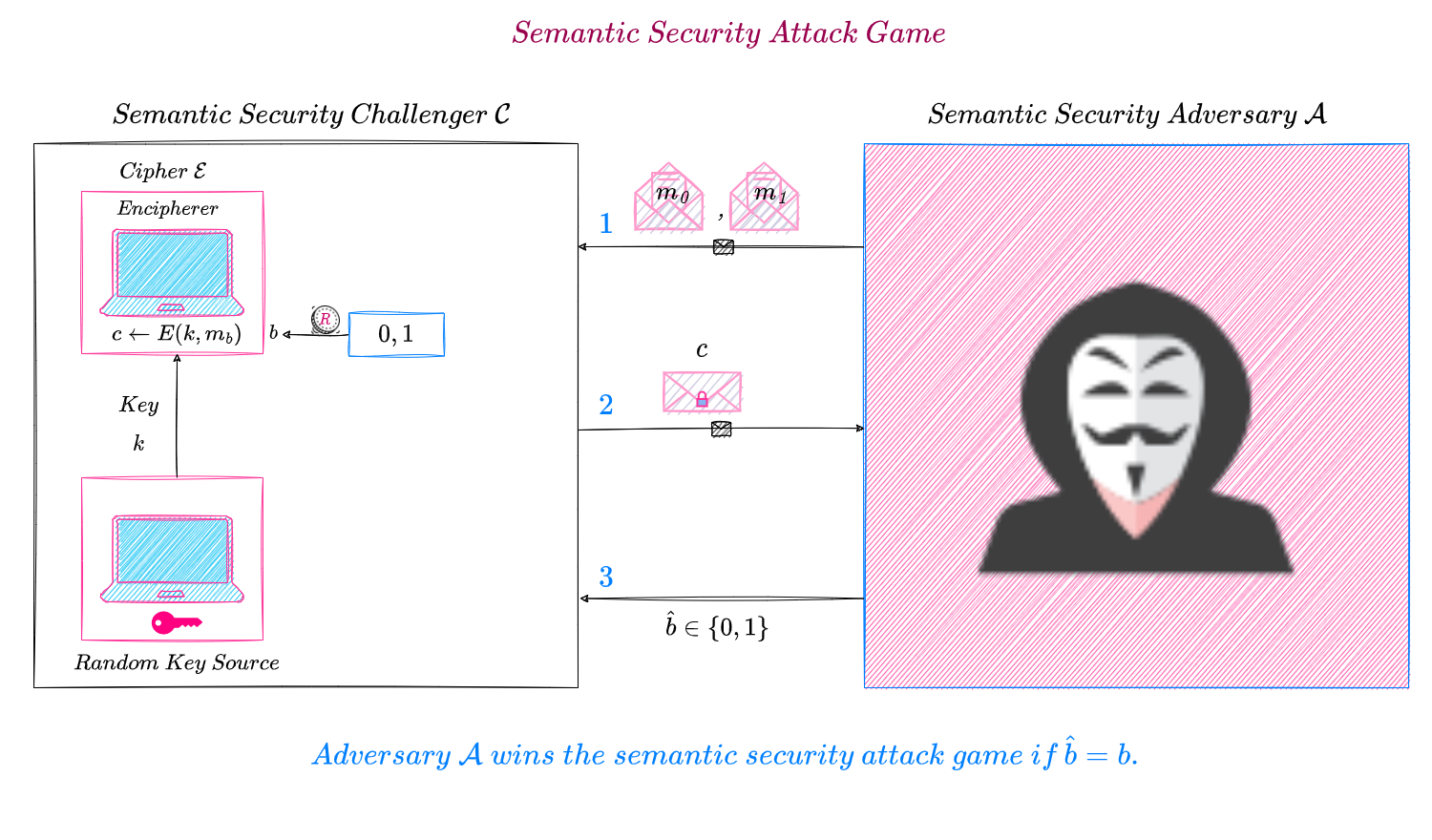
In cryptography, a game \text{G} is played between a challenger, \mathcal{C} and an adversary, \mathcal{A}, where \mathcal{A} attacks a particular notion of security of a cryptographic construct using the output generated and presented to it by \mathcal{C} (for example, \mathcal{A} attacks the semantic security of a cipher using the ciphertext generated and presented to it by \mathcal{C}).
The challenger, \mathcal{C}, generates the output by first making a random choice from a uniform distribution of possible choices as determined by the specific notion of security under attack. \mathcal{C}, subsequently uses that choice in two ways :
- as input to the cryptographic construct to generate the output (for example, in a semantic security attack game, the challenger chooses a message at random from a uniform distribution of two messages given to it by the adversary and using the chosen message as input to the cipher’s encryption algorithm produces a ciphertext as output)
- to choose between a random value and an output of a cryptographic construct (for example, in a PRG attack game, the challenger chooses uniformly and randomly between either 0 \text{ or } 1 and based on this choice outputs either a random value or a pseudo-random value which is the output of a PRG).
The adversary, \mathcal{A}, wins the game if it correctly deduces the choice made by the challenger, \mathcal{C}, that resulted in that output, otherwise it loses (for example, in the semantic security attack game, \mathcal{A} wins if, from the given ciphertext, it can correctly deduce which message was chosen by the challenger).
The following diagram illustrates a semantic security attack game.
A cryptographic construct that is insecure against a particular notion of security attack, on given an input will produce an output drawn from a non-uniform distribution of possible outputs; in fact, some outputs will have 0 probability of occurring for the given input and would be detectable by the adversary \mathcal{A} with a high (non-negligible) probability, thereby enabling it to win.
Suppose a cipher is not secure under the notion of semantic security i.e., is semantically insecure, then, a ciphertext output by this cipher would not decrypt to some messages in the message space and this non-uniform distribution of messages that resulted in the ciphertext will be noticeable by \mathcal{A} i.e., computationally distinguishable from a uniform distribution of messages that could result in that ciphertext, that is, every message sampled from this distribution is equally likely to be the encryption of that ciphertext; hence, when given a ciphertext which is the encryption of one of two possible messages, \mathcal{A} can detect with non-negligible probability that a given ciphertext could not be the encryption of one of the two messages that \mathcal{A} gave the challenger, \mathcal{C}, thereby enabling \mathcal{A} to correctly detect which one of the two messages was encrypted and consequently, win the game with a non-negligible advantage with respect to the challenger.
It should be noted that the challenger chooses uniformly and randomly from the set of possible choices so that the adversary does not win by knowing the preference of the challenger in making a particular choice but wins only when the cryptographic construct is insecure, i.e., the construct creates a non-uniform distribution of input choices for its output which could be exploited by the adversary. In other words, every cryptographic game is designed such that the adversary, \mathcal{A}, wins only by exploiting the bias of the cryptographic construct and not that of the challenger.
The input choices available to the challenger, \mathcal{C}, the method of making a choice from the available ones and the implementation of the cryptographic construct are known to the adversary, \mathcal{A}. However, the challenger, \mathcal{C}, is incognizant of the strategy used by the adversary, \mathcal{A}, to attack it.
It should be noted that \mathcal{A} is an efficient adversary i.e., its running time is poly-bounded with over-whelming probability.
The challenger, \mathcal{C}, may make its choice from a set of two or more choices, as enumerated below :
(i) uniformly at random from a set of 2 possible choices
Suppose b \in \{0, 1\} denotes the choice made by the challenger, \mathcal{C}, and \hat{b} \in \{0, 1\} denotes the adversary \mathcal{A} \text{'s} guess of the choice made by the challenger. \mathcal{A} wins when \hat{b} = b, otherwise \mathcal{C} wins and consequently, \mathcal{A} loses. Hence,
\begin{equation*}
\begin{split}
\text{G}\bold{adv}[\mathcal{A, C}] &= \text{Pr}[\mathcal{A} \text{ wins}] - \text{Pr}[\mathcal{C} \text{ wins}] \\
& = \text{Pr}[\mathcal{A} \text{ wins}] - \text{Pr}[\mathcal{A} \text{ loses}] \\
&= \text{Pr}[\hat{b} = b] - \text{Pr}[\hat{b} \neq b] \\
&= \text{Pr}[\hat{b} = b] - \text{Pr}[\hat{b} = \,\sim\!b] \\
\end{split}
\end{equation*}
Suppose, if \text{G}\bold{adv}[\mathcal{A, C}] is negative \big(\mathcal{A} loses more often than it wins\big) i.e., \text{Pr}[\hat{b} = \,\sim\!b] > \text{Pr}[\hat{b} = b] , then \text{G}\bold{adv}[\mathcal{A, C}] can be made positive by making \mathcal{A} output \sim\! \hat{b} instead of \hat{b} and it wins when \sim \!\hat{b} = b or equivalently, \hat{b} = \sim \!b. Therefore,
\begin{equation*}
\begin{split}
\text{G}\bold{adv}[\mathcal{A, C}] &= \text{Pr}[\mathcal{A} \text{ wins}] - \text{Pr}[\mathcal{A} \text{ loses}] \\
&= \text{Pr}[\hat{b} = \,\sim\!b] - \text{Pr}[\hat{b} = b] \\
\end{split}
\end{equation*}
Whenever an adversary has to choose between \bold{two} possible choices, when he gets information that he made the wrong choice, it is equivalent to getting information about the right choice. Hence in such games (as shown by the above two equations), the advantage of adversary, \mathcal{A}, over the challenger, \mathcal{C}, is defined as,
\begin{equation*}
\begin{split}
\text{G}\bold{adv}[\mathcal{A, C}] &= \big|\text{Pr}[\mathcal{A} \text{ wins}] - \text{Pr}[\mathcal{C} \text{ wins}] \big| \\
&=\big|\text{Pr}[\mathcal{A} \text{ wins}] - \text{Pr}[\mathcal{A} \text{ loses}] \big| \\
\end{split}
\end{equation*}
That is, the advantage of \mathcal{A} over \mathcal{C} is the \bold{absolute} difference in probabilities of \mathcal{A} winning the game and \mathcal{C} winning the game.
Here,
\begin{equation*}
\begin{split}
 \text{Pr}[\mathcal{A} \text{ wins}] &= \text{Pr}[b = 0]\, \text{Pr}[\hat{b} = 0 \,|\, b = 0] \\
&\hspace{0.3cm} + \,\text{Pr}[b = 1]\, \text{Pr}[\hat{b} = 1 \,|\, b = 1]\\
&=\dfrac{1}{2} \Big(1 - \text{Pr}[\hat{b} = 1 \,|\, b = 0] + \text{Pr}[\hat{b} = 1 \,|\, b = 1]\Big) \\    \\
\text{Pr}[\mathcal{A} \text{ loses}] &= \text{Pr}[b = 0]\, \text{Pr}[\hat{b} = 1 \,|\, b = 0] \\
&\hspace{0.3cm} + \,\text{Pr}[b = 1]\, \text{Pr}[\hat{b} = 0 \,|\, b = 1] \\
&= \dfrac{1}{2} \Big(\text{Pr}[\hat{b} = 1 \,|\, b = 0] + 1 -\text{Pr}[\hat{b} = 1 \,|\, b = 1]\Big) \\
\end{split}
\end{equation*}
Hence,
\begin{equation*}
\begin{split}
  \text{G}\bold{adv}[\mathcal{A, C}] &= \big|\text{Pr}[\mathcal{A} \text{ wins}] - \text{Pr}[\mathcal{A} \text{ loses}] \big| \\
&= \dfrac{1}{2} \Big|-2\, \text{Pr}[\hat{b} = 1 \,|\, b = 0] + 2\, \text{Pr}[\hat{b} = 1 \,|\, b = 1]\Big| \\
&= \Big|- \big(\text{Pr}[\hat{b} = 1 \,|\, b = 0] - \text{Pr}[\hat{b} = 1 \,|\, b = 1]\big)\Big| \\
&= \Big|\text{Pr}[\hat{b} = 1 \,|\, b = 0] - \text{Pr}[\hat{b} = 1 \,|\, b = 1]\Big| \\
\end{split}
\end{equation*}
Also,
\begin{equation*}
\begin{split}
\text{G}\bold{Bias}[\mathcal{A, C}] &= \text{Pr}[\mathcal{A} \text{ wins against } \mathcal{C} \text{ using its strategy to make a choice}]\\
&\hspace{0.4cm} - \text{Pr}[\mathcal{A} \text{ wins against } \mathcal{C} \text{ by making a choice uniformly and randomly}]\\
&  = \text{Pr}[\mathcal{A} \text{ wins}] - \dfrac{1}{2} \\
&= \text{Pr}[\hat{b} = b] - \dfrac{1}{2} \\
\end{split}
\end{equation*}
where \text{Pr}[\mathcal{A} \text{ wins}] denotes the probability that \mathcal{A} \text{ wins against } \mathcal{C} \text{ using its strategy to make a choice}.
\text{If }\text{Pr}[\hat{b} = b] < \dfrac{1}{2}, \text{ then } \text{G}\bold{Bias}[\mathcal{A, C}] < 0.
Also, when \text{Pr}[\hat{b} = b] < \dfrac{1}{2}, \text{Pr}[\hat{b} = \,\sim\!b] = 1 - \text{Pr}[\hat{b} = b] > \dfrac{1}{2}. Hence when adversary \mathcal{A} changes its strategy to win by outputting \sim\!\hat{b},
\begin{equation*}
\begin{split}
 \text{G}\bold{Bias}[\mathcal{A, C}] &= \text{Pr}[\mathcal{A} \text{ wins}] - \dfrac{1}{2} \\
&= \text{Pr}[\sim\!\hat{b} = b] - \dfrac{1}{2} \\
&= \text{Pr}[\hat{b} = \sim\!b] - \dfrac{1}{2} \\
&= 1 - \text{Pr}[\hat{b} = b] - \dfrac{1}{2} \\
&= \dfrac{1}{2} - \text{Pr}[\hat{b} = b] \\
\end{split}
\end{equation*}
Hence,
\text{G}\bold{Bias}[\mathcal{A, C}] = \Big|\text{Pr}[\mathcal{A} \text{ wins}] - \dfrac{1}{2}\Big| Also, we have already derived that,
\text{G}\bold{adv}[\mathcal{A_1, A_2}] = 2\,\big(\text{G}\bold{Bias}[\mathcal{A_1, A_2}] + \text{Pr}[\mathcal{A_1} \text{wins } \text{by making a choice uniformly and randomly}]\big) - 1 Here \mathcal{A_1 = A, A_2 = C} and \text{Pr}[\mathcal{A_1} \text{ wins by making a choice uniformly and randomly}] = \dfrac{1}{2}. Hence,
\begin{equation*}
\begin{split}
\text{G}\bold{adv}[\mathcal{A, C}] &= 2\,\Bigg(\!\text{G}\bold{Bias}[\mathcal{A, C}] + \dfrac{1}{2}\Bigg) - 1 \\
&= 2\,\text{G}\bold{Bias}[\mathcal{A,C}] \\
\end{split}
\end{equation*}
Alternatively, we can think of this relationship in another way. Since,
\text{G}\bold{Bias}[\mathcal{A, C}] = \Big|\text{Pr}[\mathcal{A} \text{ wins}] - \dfrac{1}{2}\Big| \text{Pr}[\mathcal{A} \text{ wins}] - \dfrac{1}{2} = \pm \, \text{G}\bold{Bias}[\mathcal{A, C}]\begin{equation*}
\begin{split}
\text{Pr}[\mathcal{A} \text{ wins}] &= \pm \, \text{G}\bold{Bias}[\mathcal{A, C}] + \dfrac{1}{2} \\
\text{Pr}[\mathcal{A} \text{ loses}] &= 1 - \text{Pr}[\mathcal{A} \text{ wins}] \\
&= 1 -\!\Bigg(\pm \, \text{G}\bold{Bias}[\mathcal{A, C}] + \dfrac{1}{2}\Bigg)\\
&= \dfrac{1}{2} - \!\Big(\pm \, \text{G}\bold{Bias}[\mathcal{A, C}]\Big) \\
\end{split}
\end{equation*} \begin{equation*}
\begin{split}
\text{G}\bold{adv}[\mathcal{A, C}] &= \big|\text{Pr}[\mathcal{A} \text{ wins}] - \text{Pr}[\mathcal{A} \text{ loses}] \big | \\
&= \Bigg|\pm \, \text{G}\bold{Bias}[\mathcal{A, C}] + \dfrac{1}{2} - \Bigg[\dfrac{1}{2} - \!\Big(\pm \, \text{G}\bold{Bias}[\mathcal{A, C}]\Big)\Bigg] \Bigg| \\
& = \Bigg| 2\, \Big(\pm \, \text{G}\bold{Bias}[\mathcal{A, C}]\Big) \Bigg| \\
&= 2\,\Big|\pm \text{G}\bold{Bias}[\mathcal{A, C}]\Big| \\
&= 2\,\text{G}\bold{Bias}[\mathcal{A, C}] \\
\end{split}
\end{equation*} (ii) uniformly at random from a set of N possible choices, where N > 2 and is a poly-bounded positive integer.
Whenever an adversary has to make a choice from N possible choices, getting information that he made the wrong choice i.e., lost the game, does not reveal the right choice since there are still N-1 other possible right choices. Hence in such games, the adversary cannot win by changing his strategy based on the information that he has lost the game. Therefore, the advantage of adversary, \mathcal{A}, over the challenger, \mathcal{C}, is defined as,
\begin{equation*}
\begin{split}
  \text{G}\bold{adv}[\mathcal{A, C}] &= \text{Pr}[\mathcal{A} \text{ wins}] - \text{Pr}[\mathcal{C} \text{ wins}] \times \dfrac{1}{N-1} \\
 &= \text{Pr}[\mathcal{A} \text{ wins}] - \text{Pr}[\mathcal{A} \text{ loses}] \times \dfrac{1}{N-1}\\
\end{split}
\end{equation*}
Suppose b \in \{0,\ldots, N\} denotes the input choice made by the challenger, \mathcal{C}, and \hat{b} denotes the adversary \mathcal{A} \text{'s guess of the choice made by challenger, } \mathcal{C} \text{; } \mathcal{A} wins when \hat{b} = b, otherwise \mathcal{C} wins and consequently, \mathcal{A} loses. Hence,
\begin{equation*}
\begin{split}
 \text{G}\bold{adv}[\mathcal{A, C}] &= \text{Pr}[\mathcal{A} \text{ wins}] - \text{Pr}[\mathcal{A} \text{ loses}] \times \dfrac{1}{N-1} \\
&= \text{Pr}[\mathcal{A} \text{ wins}] - \big(1 - \text{Pr}[\mathcal{A} \text{ wins}]\big) \times \dfrac{1}{N-1} \\
&= \text{Pr}[\mathcal{A} \text{ wins}] \Big(1 +\dfrac{1}{N-1} \Big) - \dfrac{1}{N-1} \\
&= \text{Pr}[\mathcal{A} \text{ wins}] \times \dfrac{N}{N-1} - \dfrac{1}{N-1}\\
&= \text{Pr}[\hat{b} = b] \times \dfrac{N}{N-1} - \dfrac{1}{N-1} \\
\end{split}
\end{equation*}
Also,
\begin{equation*}
\begin{split}
\text{G}\bold{Bias}[\mathcal{A, C}] &= \text{Pr}[\mathcal{A} \text{ wins against } \mathcal{C} \text{ using its strategy to make a choice}]\\
&\hspace{0.4cm} - \text{Pr}[\mathcal{A} \text{ wins against } \mathcal{C} \text{ by making a choice uniformly and randomly}]\\
&= \text{Pr}[\mathcal{A} \text{ wins}] - \dfrac{1}{N} \\
&= \text{Pr}[\hat{b} = b] - \dfrac{1}{N} \\
\end{split}
\end{equation*}
where \text{Pr}[\mathcal{A} \text{ wins}] denotes the probability that \mathcal{A} \text{ wins against } \mathcal{C} \text{ using its strategy to make a choice}.
Summary
In a game \text{G}, when the challenger, \mathcal{C}, makes its choice
(i) uniformly and randomly from a set of 2 possible choices
the advantage of adversary, \mathcal{A}, over the challenger, \mathcal{C}, is defined as,
\begin{equation*}
\begin{split}
\text{G}\bold{adv}[\mathcal{A, C}] &= \big|\text{Pr}[\mathcal{A} \text{ wins}] - \text{Pr}[\mathcal{C} \text{ wins}] \big| \\
&=\big|\text{Pr}[\mathcal{A} \text{ wins}] - \text{Pr}[\mathcal{A} \text{ loses}] \big| \\
& =\big|\text{Pr}[\mathcal{A} \text{ loses}] - \text{Pr}[\mathcal{A} \text{ wins}] \big| \\
&= \Big|\text{Pr}[\hat{b} = 1 \,|\, b = 0] - \text{Pr}[\hat{b} = 1 \,|\, b = 1]\Big| \\
\end{split}
\end{equation*}
where, b \in \{0, 1\} denotes the input choice made by the challenger, \mathcal{C}, and \hat{b} \in \{0, 1\} denotes the adversary \mathcal{A} \text{'s output}. \mathcal{A} wins when \hat{b} = b, otherwise \mathcal{C} wins and consequently, \mathcal{A} loses.
The bias of adversary \mathcal{A} is given by,
\begin{equation*}
\begin{split}
\text{G}\bold{Bias}[\mathcal{A, C}] &= \text{Pr}[\mathcal{A} \text{ wins against } \mathcal{C} \text{ using its strategy to make a choice}]\\
&\hspace{0.4cm} - \text{Pr}[\mathcal{A} \text{ wins against } \mathcal{C} \text{ by making a choice uniformly and randomly}]\\
&= \bigg|\text{Pr}[\mathcal{A} \text{ wins}] - \dfrac{1} {2}\bigg| \\
\end{split}
\end{equation*}
where \text{Pr}[\mathcal{A} \text{ wins}] denotes the probability that \mathcal{A} \text{ wins against } \mathcal{C} \text{ using its strategy to make a choice}.
Also,
\text{G}\bold{adv}[\mathcal{A, C}] = 2\,\text{G}\bold{Bias}[\mathcal{A,C}] (ii) uniformly and randomly from a set of N possible choices, where N > 2 and is a poly-bounded positive integer.
the advantage of adversary, \mathcal{A}, over the challenger, \mathcal{C}, is defined as,
\begin{equation*}
\begin{split}
\text{G}\bold{adv}[\mathcal{A, C}] &= \text{Pr}[\mathcal{A} \text{ wins}] - \text{Pr}[\mathcal{C} \text{ wins}] \times \dfrac{1}{N-1}\\
&= \text{Pr}[\mathcal{A} \text{ wins}] - \text{Pr}[\mathcal{A} \text{ loses}] \times \dfrac{1}{N-1}\\
&= \text{Pr}[\mathcal{A} \text{ wins}] - \big(1 - \text{Pr}[\mathcal{A} \text{ wins}]\big) \times \dfrac{1}{N-1} \\
&= \text{Pr}[\hat{b} = b] \times \dfrac{N}{N-1} - \dfrac{1}{N-1} \\
\end{split}
\end{equation*}
where b \in \{0,\ldots, N\} denotes the choice made by the challenger, \mathcal{C}, and \hat{b} denotes the output of the adversary \mathcal{A}. \mathcal{A} wins when \hat{b} = b, otherwise \mathcal{C} wins and consequently, \mathcal{A} loses.
The bias of adversary \mathcal{A} is given by,
\begin{equation*}
\begin{split}
\text{G}\bold{Bias}[\mathcal{A, C}] &= \text{Pr}[\mathcal{A} \text{ wins against } \mathcal{C} \text{ using its strategy to make a choice}]\\
&\hspace{0.4cm} - \text{Pr}[\mathcal{A} \text{ wins against } \mathcal{C} \text{ by making a choice uniformly and randomly}]\\
&= \text{Pr}[\mathcal{A} \text{ wins}] - \dfrac{1}{N} \\
&= \text{Pr}[\hat{b} = b] - \dfrac{1}{N} \\
\end{split}
\end{equation*}
where \text{Pr}[\mathcal{A} \text{ wins}] denotes the probability that \mathcal{A} \text{ wins against } \mathcal{C} \text{ using its strategy to make a choice}.