\begin{equation*}
\begin{split}
\textit{Distinguishing Advantage} & = \big|\text{Advantage of Adversary with respect to Challenger}\big| \\
& = \big|\text{Probability that the Adversary wins - Probability that the Challenger wins} \big| \\
& = \big|\text{Probability that the Adversary wins - Probability that the Adversary loses} \big| \\
\end{split}
\end{equation*}
For a deep intuitive understanding of advantage refer to this and this.
Why is the advantage an absolute value? It suggests that even when the adversary loses more than it wins, it has an advantage. Why is this so?
Let us consider the following example to answer these questions.
Suppose we have a loaded coin with a bias of \frac{1}{4} towards head. For this coin, the probability of heads, P(H) = \frac{1}{2} + bias = \frac{1}{2} + \frac{1}{4} = \frac{3}{4} and the probability of tails, P(T) = \frac{1}{2} - bias = \frac{1}{2} - \frac{1}{4} = \frac{1}{4}.
Now you play a game in the casino. The casino asks you to choose either Heads or Tails, and you win whenever what you choose turns up. No casino would ever play this game with the loaded coin we just described (as if life is that kind! 😂), but for the purpose of this example let us assume that’s the case.
Let us assume that you play this game several times.
Suppose you pick Heads. Now,
Your advantage with respect to the casino = Probability you win – Probability you lose (or Probability the casino wins) = \frac{3}{4} - \frac{1}{4} = \frac{1}{2}.
Now, suppose you had picked Tails. When you play this game several times, you would notice that you are winning only \frac{1}{4}th of the time. So you would eventually know that the coin is loaded in favor of Heads and you would change your strategy and pick Heads and win \frac{3}{4}th of the time and have an advantage of \frac{1}{2}. This is why the definition of advantage has an absolute sign since irrespective of whether you picked Heads or Tails, you would eventually know that the coin is loaded and hence have the same advantage in both the cases. This is the reason we define your advantage with respect to the casino as \big|Probability you win – Probability you lose (or Probability the casino wins)\big| or more generally, ‘Advantage of Adversary with respect to Challenger’ as an absolute value.
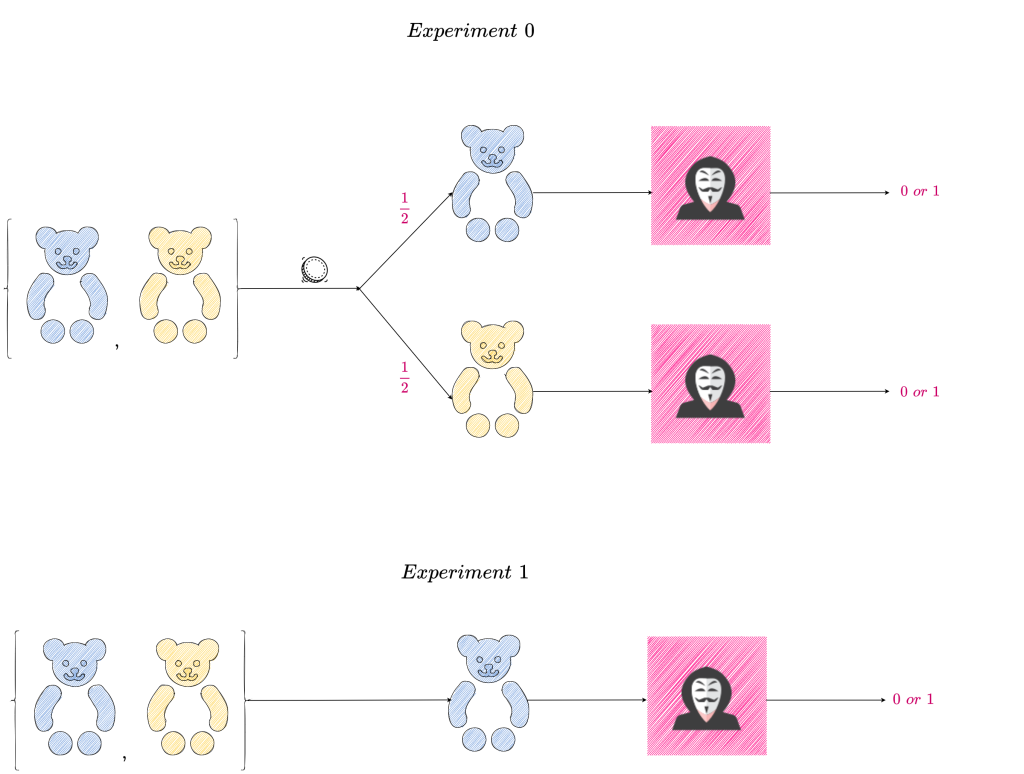
Annie is on her summer vacation and she decides to take a break from reading. Her neighbor Marie is her nemesis and so Annie devises a game to outsmart her. Annie has two bears, one blue and the other yellow. Annie’s game is as follows:
She devises two experiments – Experiment\textit{0} and Experiment\textit{1}.
In Experiment\textit{0}, Annie randomly picks a bear, with each bear having equal probability of being picked. She communicates to Marie the color of the bear she picked.
In Experiment\textit{1}, Annie always picks the blue bear and communicates the color ‘Blue’ to Marie.
Marie’s goal is to distinguish Experiment\textit{0} from Experiment\textit{1}. At the end of each experiment (i.e., when Marie receives a color from Annie), she outputs 0 or 1 as a guess for which experiment she thinks she is in. She wins if she guesses correctly, otherwise she loses.
They play this game several times.
The following diagram is a pictorial representation of the two experiments.
To distinguish between the two experiments, Marie has to maximize her distinguishing advantage. How does she do that?
Before proceeding, let us define some notations we will be using.
Let \mathcal{S = \{\textit{'Blue', 'Yellow'}\}} denote the sample space which comprises the possible outcomes of the experiments 0 \text{ and } 1.
Let E_0 \text{ and } E_1 be random variables denoting the outcome of experiments 0 \text{ and } 1 respectively.
We know that a random variable maps the sample space to a real line i.e., ‘Blue’ would be mapped to a real number and ‘Yellow’ would be mapped to another real number. But for clarity’s sake we will omit this mapping and directly deal with the values in the sample space, \mathcal{S}.
Suppose say ‘Blue’ maps to 1, then P(E_0 = 1) would denote the probability that the outcome of experiment 0 is 1 i.e., ‘Blue’ (Annie picks a ‘Blue’ bear and communicates the color ‘Blue’ to Marie). We would instead denote this probability as P(E_0 = \textit{'Blue'}), for ease of understanding.
For Marie to win, she needs to distinguish between experiments 0 \text{ and } 1. Her success in distinguishing between the two experiments depends on how different the outcomes of the two experiments are. For example, if she gets ‘Yellow’ she knows that it is the outcome of experiment 0 since it is impossible for experiment 1 to have an outcome of ‘Yellow’.
Hence her success in distinguishing between the two experiments depends on how different the probability distributions of the outcomes of the two experiments are i.e., the distance (to be precise, the total variation distance) between the distributions of E_0 \text{ and } E_1 and her ability to measure this distance accurately.
Therefore, to distinguish between experiment 0 \text{ and } 1, she tries to maximize her distinguishing advantage (or equivalently, the distinguishing distance), namely the quantity,
where \mathcal{D(\cdot)} is a distinguisher function that distinguishes between the probability distributions of E_0 \text{ and } E_1. \mathcal{D}(E_0) means \mathcal{D} takes as input \mathcal{s \in S}, where \mathcal{s} is drawn from the distribution of E_0 and outputs either 0 or 1. Similarly for \mathcal{D}(E_1). This quantity is denoted by \text{Adv}_D(E_0, E_1).
where \big\|E_0 - E_1\big\|_{TV} is the total variation distance between the probability distributions of random variables E_0 \text{ and } E_1 i.e., the probability distributions of the outcomes of experiments 0 \text{ and } 1.
From this equation, we can infer that the total variation distance between the distributions of E_0 \text{ and } E_1 maximizes the distinguishing advantage.
An alternate way to express the above equation is as follows,
where \mathcal{W_0} is the event that the adversary \mathcal{A} (Marie) outputs \mathcal{1} when given as input \mathcal{s \in S} drawn from the distribution of E_0 and \mathcal{W_1} is the event that the adversary \mathcal{A} outputs \mathcal{1} when given as input \mathcal{s \in S} drawn from the distribution of E_1.
Or expressed more succinctly, W_b is the event that Marie outputs 1 in experiment b, where b = \{0, 1\}.
Since the total variation distance between random variables E_0 \text{ and } E_1 maximizes the distinguishing advantage, in order to calculate this distance we need to construct the probability distributions of E_0 \text{ and } E_1.
This shows that the maximum advantage possible in distinguishing between the two experiments is \frac{1}{2}. Since Marie’s distinguishing advantage is due to the difference in probability distributions of the outcomes of the experiments, her distinguishing advantage cannot be more than the total variation distance between the two distributions, which is a measure of the difference between the two distributions.
The following is a pictorial representation of the probability distributions of the outcomes of experiments 0 \text{ and } 1.
The following diagram shows an alternate way to calculate total variation distance between the outcomes of experiments 0 \text{ and } 1.
The total variation distance between distributions of random variables E_0 \text{ and } E_1 denoting the outcomes of experiments 0 \text{ and } 1 respectively, can also be defined as
We have already proved that both sets \mathcal{A = \{ s \in S :\, } P(E_0 = s) \geq P(E_1 = s)\} and \mathcal{A^c = \{ s \in S :\, } P(E_0 = s) < P(E_1 = s)\} maximize \big|P(E_0 \in \mathcal{B}) - P(E_1 \in \mathcal{B}) \big|.
Here, \mathcal{A = \{\textit{'Yellow'}\}} and \mathcal{A^c = \{\textit{'Blue'}\}}. Also, the support of random variables E_0 \text{ and } E_1 is \{\textit{'Blue', 'Yellow'}\}.
We have proved mathematically that Marie’s distinguishing advantage cannot be more than \frac{1}{2}. Marie’s distinguishing advantage depends on the distinguisher function that she uses to distinguish between the two distributions. In order for Marie to maximize her distinguishing advantage, she needs to find the best distinguisher function i.e., one that maximizes her advantage.
When Annie sends a color to Marie, how does Marie construct her distinguisher function so that she maximizes her distinguishing advantage?
Before we use mathematics to construct the required distinguisher function, let us use our intuition to think through this problem and then verify the soundness of our intuition mathematically.
Since distinguishing advantage is the absolute difference in probabilities between Marie winning and Marie losing i.e.,
in order for Marie to maximize her distinguishing advantage, she needs to maximize her probability of winning (which in turn minimizes her probability of losing).
How does she maximize her probability of winning? Since she can get two colors as input namely, ‘Blue’ and ‘Yellow’ she needs to maximize her probability of winning in each case. Lets examine the two cases.
Marie gets ‘Yellow’ as input
Marie knows that she can get ‘Yellow’ as an outcome only in experiment \mathcal{0}. Hence she maximizes her probability of winning (her probability of winning is \mathcal{1}) by outputting \mathcal{0} whenever she gets ‘Yellow’ as input.
Marie gets ‘Blue’ as input
Marie can get ‘Blue’ as an outcome only both experiments i.e., in \mathcal{0 \text{ and } 1}. The probability that she gets ‘Blue’ is given by,
So when Marie gets ‘Blue’, there is a \mathcal{\frac{1}{4}} \div \frac{3}{4} = \frac{1}{4} \times \frac{4}{3} = \frac{1}{3} probability that it comes from experiment \mathcal{0} and \mathcal{\frac{2}{3}} probability that it comes from experiment \mathcal{1}. So ‘Blue’ is twice more likely to be an outcome of experiment \mathcal{1} than \mathcal{0}. Since Marie wants to maximize her probability of winning, when she gets ‘Blue’ and outputs \mathcal{1}, she is twice more likely to be correct than wrong. Hence to maximize her probability of winning she should output \mathcal{1} when she gets ‘Blue’ as input.
By this reasoning, the best distinguisher i.e., the one that maximizes her distinguishing advantage outputs \mathcal{0} when given ‘Yellow’ as input and outputs \mathcal{1} when given ‘Blue’ as input.
Since distinguishing advantage is an absolute value i.e., it only measures the distinguishability between experiments, the inverse strategy should also work. So another distinguisher which would maximize her advantage would be one that outputs \mathcal{0} when given ‘Blue’ as input and outputs \mathcal{1} when given ‘Yellow’ as input.
Any other distinguisher would give a distinguishing advantage less than what the above two distinguishers would give.
To verify this hypothesis, let us construct the following two distinguisher functions and calculate the respective advantages that they give.
Distinguisher function \mathcal{D} on getting ‘Blue’ as input outputs \mathcal{0} with probability \mathcal{\frac{1}{3}} and \mathcal{1} with probability \mathcal{\frac{2}{3}}.
Distinguisher function \mathcal{D} on getting ‘Yellow’ as input outputs \mathcal{0} with probability \mathcal{1}.
Distinguisher function \mathcal{D} on getting ‘Blue’ as input outputs \mathcal{0} with probability \mathcal{\frac{1}{2}} and \mathcal{1} with probability \mathcal{\frac{1}{2}}.
Distinguisher function \mathcal{D} on getting ‘Yellow’ as input outputs \mathcal{0} with probability \mathcal{1}.
If our reasoning is correct, the distinguishing advantage of the distinguisher described in \mathcal{(1)} will be more than that of distinguisher described in \mathcal{(2)}, since when Marie gets ‘Blue’ it is twice more likely to be the outcome of experiment \mathcal{1} than \mathcal{0}, any distinguisher that outputs \mathcal{1} with a higher probability when given ‘Blue’, will have a higher probability of winning. Hence the best distinguisher will output \mathcal{1} with probability \mathcal{1} when given ‘Blue’ as input. Since distinguisher in \mathcal{(1)} outputs \mathcal{1} with probability \mathcal{\frac{2}{3}} when given ‘Blue’ as input and distinguisher in \mathcal{(2)} outputs \mathcal{1} with probability \mathcal{\frac{1}{2}} when given ‘Blue’ as input, the distinguishing advantage we get using distinguisher in \mathcal{(1)} will be more than what we get when using distinguisher in \mathcal{(2)}\big(since ‘Blue’ occurs twice more times in experiment \mathcal{1} than \mathcal{0} and \mathcal{\frac{2}{3} > \frac{1}{2}}\big).
Let us enumerate the distinguishers we have come up with so far through our reasoning. We will calculate the distinguishing advantage of each of these distinguishers and use the definition of distinguishing advantage (which we have derived earlier) to check whether our reasoning is correct.
Since Marie can get either of ‘Blue’ or ‘Yellow’ as input,
P(\textit{'Blue'}) + P(\textit{'Yellow'}) = 1
We have already calculated P(\textit{'Blue'}) = \frac{3}{4}. Of the \frac{3}{4} times ‘Blue’ occurs \frac{1}{4} is from experiment \mathcal{0} and \frac{1}{2} is from experiment \mathcal{1}. Also,
Let us calculate the distinguishing advantage of each of the distinguishers we have described so far.The distinguisher function \mathcal{D} outputs \mathcal{0} on getting ‘Yellow’ as input and outputs \mathcal{1} on getting ‘Blue’ as input.
Since we have already proved that the distinguishing advantage cannot be greater than \frac{1}{2}, this confirms that our reasoning is correct, i.e., this distinguishing function \mathcal{D} is the best possible distinguisher.
Next lets calculate the distinguishing advantage of a distinguisher that does the inverse of the previous distinguisher, namely outputs 1 when it gets ‘Yellow’ as input and outputs 0 when it gets ‘Blue’ as input.
We had already reasoned that this distinguisher will also maximize the distinguishing advantage because it maximizes the probability of losing and consequently minimizes the probability of winning. Since distinguishing advantage is an absolute value, this distinguisher is equivalent to one that maximizes the probability of winning and consequently minimizes the probability of losing. Hence both the distinguishers have the same distinguishing advantage of \frac{1}{2} as can be seen for the calculations.
Now lets calculate the distinguishing advantage of a distinguisher \mathcal{D} that on getting ‘Yellow’ as input, outputs \mathcal{0} with probability \mathcal{1} and on getting ‘Blue’ as input, outputs \mathcal{0} with probability \mathcal{\frac{1}{3}} and \mathcal{1} with probability \mathcal{\frac{2}{3}}.
We have already discussed why the distinguishing advantage of this distinguisher must be less than the previous two distinguishers and the above calculation confirms that our reasoning is correct.
Now let us calculate the distinguishing advantage of a distinguisher that we reasoned will perform worse than previous distinguisher and verify whether this indeed is the case.
Distinguisher function \mathcal{D} on getting ‘Yellow’ as input, outputs \mathcal{0} with probability \mathcal{1} and on getting ‘Blue’ as input outputs \mathcal{0} with probability \mathcal{\frac{1}{2}} and \mathcal{1} with probability \mathcal{\frac{1}{2}}.
As expected the distinguishing advantage of this distinguisher is less than that of the previous distinguisher.
These calculations confirm that to maximize the distinguishing advantage we have to design the distinguisher in such a way that it maximizes Marie’s (adversary’s) probability of winning.
Now let us come up with the best distinguisher using mathematics and show that it would be the same distinguishers we arrived at using our reasoning.
Marie, in order to maximize her distinguishing advantage should find a distinguisher function \mathcal{D}(\cdot) that maximizes \big|P[\mathcal{D}(E_0) = 1] - P[\mathcal{D}(E_1) = 1]\big|.
She can maximize her distinguishing advantage in the following four ways :
In order to maximize the difference \big|P[\mathcal{D}(E_0) = 1] - P[\mathcal{D}(E_1) = 1]\big|, Marie minimizes P[\mathcal{D}(E_1) = 1] and checks what is the maximum value P[\mathcal{D}(E_0) = 1] can take.
Since Marie tries to minimize P[\mathcal{D}(E_1) = 1] and the minimum value it can take is 0, let P[\mathcal{D}(E_1) = 1] = 0.
P[\mathcal{D}(E_1) = 1] = 0 when the distinguisher outputs 0 when it gets ‘Blue’ as input.
When the distinguisher gets ‘Yellow’ as input, it can either output 0 \text{ or } 1. Let us see what happens in each case.
(i) Distinguisher outputs 0 when it gets ‘Yellow’ as input.
P[\mathcal{D}(E_0) = 1] is the probability that the distinguisher outputs 1, given an input (or sample drawn) from experiment 0. Since this distinguisher always outputs 0, irrespective of whether it gets ‘Blue’ or ‘Yellow’ as input, P[\mathcal{D}(E_0) = 1] = 0\big(The factor of \frac{1}{2} is due to experiment 0 getting ‘Blue’ with probability \frac{1}{2} and ‘Yellow’ also with probability \frac{1}{2}\big).
The distinguishing advantage of a distinguisher that outputs 0 when given ‘Blue’ as input and 1 when given ‘Yellow’ as input is \frac{1}{2}.
In order to maximize the difference \big|P[\mathcal{D}(E_0) = 1] - P[\mathcal{D}(E_1) = 1]\big|, Marie maximizes P[\mathcal{D}(E_1) = 1] and checks what is the minimum value P[\mathcal{D}(E_0) = 1] can take.
Since Marie tries to maximize P[\mathcal{D}(E_1) = 1] and the maximum value it can take is 1, let P[\mathcal{D}(E_1) = 1] = 1.
P[\mathcal{D}(E_1) = 1] = 1 when the distinguisher outputs 1 when it gets ‘Blue’ as input.
When the distinguisher gets ‘Yellow’ as input, it can either output 0 \text{ or } 1. Let us see what happens in each case.
(i) Distinguisher outputs 0 when it gets ‘Yellow’ as input.
The distinguishing advantage of a distinguisher that always outputs 1 is 0.
In order to maximize the difference \big|P[\mathcal{D}(E_0) = 1] - P[\mathcal{D}(E_1) = 1]\big|, Marie minimizes P[\mathcal{D}(E_0) = 1] and checks what is the maximum value P[\mathcal{D}(E_1) = 1] can take.
Since Marie tries to minimize P[\mathcal{D}(E_0) = 1] and the minimum value it can take is 0, let P[\mathcal{D}(E_0) = 1] = 0.
P[\mathcal{D}(E_0) = 1] = 0 when the distinguisher always outputs 0. This is the distinguisher we have discussed in (1) (i) and its distinguishing advantage is 0.
In order to maximize the difference \big|P[\mathcal{D}(E_0) = 1] - P[\mathcal{D}(E_1) = 1]\big|, Marie maximizes P[\mathcal{D}(E_0) = 1] and checks what is the minimum value P[\mathcal{D}(E_1) = 1] can take.
Since Marie tries to maximize P[\mathcal{D}(E_0) = 1] and the maximum value it can take is 1, let P[\mathcal{D}(E_0) = 1] = 1.
P[\mathcal{D}(E_0) = 1] = 1 when the distinguisher always outputs 1. This is the distinguisher we have discussed in (2) (ii) and its distinguishing advantage is 0.
The distinguishers that maximize the distinguishing advantage are the ones in the cases (1) (ii) \text{ and } (2) (i). These are the same distinguishers we came up with through our reasoning.
Let us use the alternate notation used in defining distinguishing advantage and come up with the best distinguisher. Obviously this definition would also give us the same distinguishers we had already come up with. Let us do this exercise to convince ourselves that the two definitions are indeed equivalent (we have already proved their equivalence mathematically) and also more importantly so that we are fluent in using both these definitions.
Since we have already expounded on how to come up with the best distinguisher, this discussion will be succinct.
where W_b is the event that Marie outputs 1 in experiment b, where b = \{0, 1\}.
As already discussed, we can maximize the distinguishing advantage, \mathcal{\big|P[\mathcal{W_0}] - P[\mathcal{W_1}]\big|} in four ways.
In order to maximize the distinguishing advantage, \mathcal{\big|P[\mathcal{W_0}] - P[\mathcal{W_1}]\big|}, Marie minimizes P[\mathcal{W_1}] and checks what is the maximum value P[\mathcal{W_0}] can take.
Since Marie tries to minimize P[\mathcal{W_1}] and the minimum value it can take is 0, let P[\mathcal{W_1}] = 0.
P[\mathcal{W_1}] = 0 means the probability that Marie outputs 1 in experiment 1 is 0. For this to be true Marie has to output 0 when she gets ‘Blue’ as input.
When Marie gets ‘Yellow’ as input, she can either output 0 \text{ or } 1. Let us see what happens in each case.
(i) Marie outputs 0 when she gets ‘Yellow’ as input.
P[\mathcal{W_0}] is the probability that Marie outputs 1, given an input (or sample drawn) from experiment 0. Since Marie always outputs 0, irrespective of whether she gets ‘Blue’ or ‘Yellow’ as input, P[\mathcal{W_0}] = 0\big(The factor of \frac{1}{2} is due to experiment 0 getting ‘Blue’ with probability \frac{1}{2} and ‘Yellow’ also with probability \frac{1}{2}\big).
The distinguishing advantage of an adversary who always outputs 0 when given ‘Blue’ as input and 1 when given ‘Yellow’ as input is \frac{1}{2}.
We can see that this definition of distinguishing advantage gives us the exact same distinguishers we got using the previous definition of distinguishing advantage \Big(\big|P[\mathcal{D}(E_0) = 1] - P[\mathcal{D}(E_1) = 1]\big|\Big). We can work through the other cases in a similar way as we have done using the previous definition. Hence we will omit working through the other cases.
Summary
The purpose of this exercise is to show that the distinguishing advantage of the adversary is derived from the probability distributions of the outcomes of the two experiments being different and the adversary’s ability to measure it.
What happens when the probability distributions of the outcomes of the two experiments are different but the adversary is unable to measure it? Then for all practical purposes the two experiments are indistinguishable and the distinguishing advantage of the adversary would be negligible. (Refer here to refresh why indistinguishability of distributions matters in cryptography.) When we design secure cryptographic systems it is only required that all efficient adversaries have a negligible advantage. So what do these terms “negligible” and “efficient” mean? And more importantly what does it mean for a cryptographic system to be secure? This is the next topic of our discussion. This is the central tenet of cryptography and all subsequent knowledge would be moot without a thorough understanding of the meaning of security as applied to cryptography.
Let us return to the story of John and his identical twin sisters Ann and Kelly. John has 1 kg of gold which he would like to divide between his two sisters.
We will consider two possible scenarios. In one, John loves both his sisters equally and hence is unbiased towards them; in another, John is a bit disappointed about Kelly’s foray into the fashion influencer world and hence loves Ann more than Kelly i.e., he is biased towards Ann.
Let us see how bias and advantage plays out in these two scenarios.
Let us first consider the case where John is unbiased.
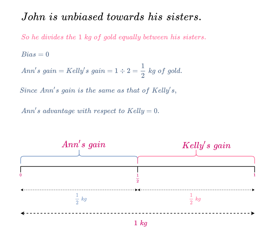
Since John is unbiased (i.e., bias = 0) , he divides the 1 kg of gold equally between his sisters. So each sister gets 1 \div 2 = \frac{1}{2} kg of gold. What is the advantage in being Ann rather than Kelly? Since both Ann’s gain and Kelly’s gain are the same (\frac{1}{2} kg of gold), there is no advantage in being Ann rather than Kelly. So the advantage of Ann with respect to Kelly = 0.
The following is a pictorially representation of the scenario when John is unbiased.
Now let us consider the case where John is biased towards Ann.
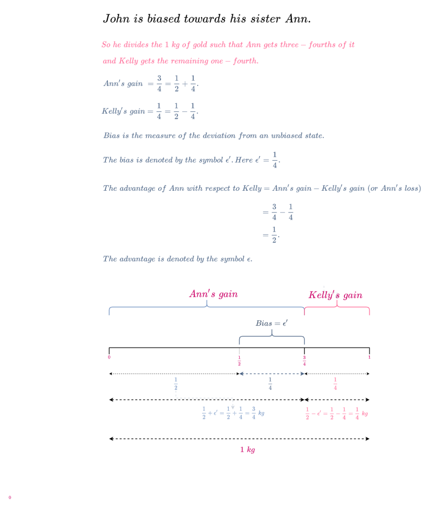
Since John loves Ann more than Kelly, he divides the 1 kg of gold such that Ann gets \frac{3}{4} kg of gold and Kelly gets the remaining \frac{1}{4} kg of gold. Due to John’s bias, Ann now gets \frac{1}{4} kg of more gold and Kelly gets \frac{1}{4} kg of less gold compared to John’s unbiased state, when they each got \frac{1}{2} kg of gold.
Bias is a measure of the deviation from the unbiased state (where the gold was divided equally between the two sisters).
Ann’s gain = Unbiased Gain + bias = \frac{1}{2} + \frac{1}{4} = \frac{3}{4} kg.
Kelly’s gain = Unbiased Gain - bias = \frac{1}{2} - \frac{1}{4} = \frac{1}{4} kg.
Due to John favoring Ann over Kelly, Ann enjoys a positive bias of \frac{1}{4} and consequently, Kelly suffers from a negative bias of \frac{1}{4}.
The bias is denoted by the symbol \epsilon^\prime. Here \epsilon^\prime = \frac{1}{4}.
Is there an advantage of being Ann rather than Kelly? We can answer this question by finding out who is richer i.e., who gained more.
The advantage of Ann with respect to Kelly = Ann’s gain - Kelly’s gain = \frac{3}{4} - \frac{1}{4} = \frac{1}{2}.
Since Ann gained \frac{1}{2} kg more gold than Kelly, in this scenario there is a clear advantage in being Ann.
So we can define the advantage of one person with respect to another person in a game as the difference in gains between the two persons.
When Kelly gains \frac{1}{4} kg of gold, it is equivalent to Ann losing \frac{1}{4} kg of gold since she doesn’t get Kelly’s share. Had Kelly not been there, Ann would have got the entire 1 kg to gold. So missing out on the \frac{1}{4} kg of gold due to Kelly can be viewed as Ann’s loss.
Since when one person losses the other person gains we can also define advantage as follows.
The advantage of one person with respect to another person in a game can also we viewed as the difference between the gains and losses of the same person.
Using this definition,
The advantage of Ann with respect to Kelly = Ann’s Gain - Ann’s Loss = \frac{3}{4} - \frac{1}{4} = \frac{1}{2}.
We see that this agrees with our previous definition of advantage.
We see that the advantage is twice the bias. Why is this so?
When Ann gains \frac{3}{4} kg of gold, her gain is equivalent to \Big(\frac{1}{2} + \frac{1}{4}\Big) kg of gold and her loss is 1 - \Big(\frac{1}{2} + \frac{1}{4}\Big) = \Big(\frac{1}{2} - \frac{1}{4}\Big) kg of gold.
Intuitively this makes sense because when one person’s gain is \frac{1}{2} + \epsilon^\prime then that person’s loss (or the other person’s gain) is 1 - \Big(\frac{1}{2} + \epsilon^\prime\Big) = \frac{1}{2} - \epsilon^\prime and so the advantage, \epsilon, which is defined as the difference between their respective gains becomes \Big(\frac{1}{2} + \epsilon^\prime\Big) - \Big(\frac{1}{2} -\epsilon^\prime\Big) = 2\epsilon^\prime .
The following is a pictorial representation of the case where John is biased.
Ann’s hedge fund decides to invest in movies and Ann has to move to Los Angeles for 6 months to meet with Hollywood production houses and make deals. Meanwhile Kelly is growing immensely successful as a fashion influencer and has been offered a role in the documentary “The Lives of Famous Wenches”. She would be shooting in Los Angeles for 8 months.
Ann is in New York from January to June and for the remaining 6 months (July to December) she is in Los Angeles. Kelly is in New York from January to April and for the remaining 8 months (May to December) she is in Los Angeles.
The following table pictorially represents their whereabouts throughout the year.
As Kelly’s fame grows, she is getting noticed by an underworld criminal network, who wants to kidnap her for ransom. Meanwhile Michael, an out of work hitman (in this era of cancel culture why would a person need to be murdered to be done away with, when all that is required is to assassinate his character), feeling maudlin with self pity, is hired for the job. The underworld don contacts Michael and asks him to kidnap Kelly, providing him with a photo of Kelly and also information about when Kelly would be in New York and when she would be in Los Angles. The don is however unaware of Kelly’s identical twin sister, Ann, and hence Michael is also ignorant of Ann’s existence. Also Michael will kidnap Kelly at the most opportune time when he is sure that he would not be caught by the police.
Since Michael runs some risk of getting caught by the police, he wants to know whether he has an advantage in this kidnapping game. Does he succeed with a higher probability than if he had just succeeded at random?
Before answering these questions, let us take a little detour to understand some important concepts like bias and advantage with an intuitive example. We will then connect these concepts to the story of statistical distance.
Note: It is of paramount importance to understand bias and advantage as they form the basis of many security proofs in cryptography. If you are already familiar with these concepts you can continue reading, though I would still prefer that the reader peruses the example so that we are on the same page.
Now that we are familiar with advantage and bias, let us use these concepts to answer whether Michael has an advantage with respect to Kelly. We can view the kidnapping as a game with two participants, namely, Michael and Kelly. If Michael wins the game it means that he successfully kidnaps Kelly and hence he wins and Kelly loses. On the contrary, if Michael loses it means that he fails to kidnap Kelly and hence Kelly wins.
\begin{equation*}
\begin{split}
\textit{Advantage of Michael with respect to Kelly} & = \textit{Probability that Michael Wins - Probability that Kelly Wins} \\
& = \textit{Probability that Michael Wins - Probability that Michael Loses}\\
\end{split}
\end{equation*}
In order to calculate Michael’s advantage over Kelly, let us first calculate his probability of winning and losing.
The following discussion assumes knowledge about some basic concepts in probability as discussed in Probability Primer.
Let W be the event that Michael wins (i.e., he successfully kidnaps Kelly) given that Ann and Kelly look alike (since they are identical twins), Michael is ignorant of Ann’s existence and Michael knows Kelly’s schedule. In how many ways can this event occur? Michael can kidnap Kelly anytime between January and December.
Let W_1 denote the event that Michael successfully kidnaps Kelly between January and December. What is the probability that he succeeds? During this time, Ann and Kelly are both in New York; and, since Ann and Kelly are identical twins, Michael can succeed only by making a random guess i.e., his probability of success is \frac{1}{2}. The probability that he successfully kidnaps Kelly in January is the probability that he kidnaps Kelly in January times the probability that he kidnaps Kelly i.e., \frac{1}{12} \times \frac{1}{2} So during the 4 months between January to April (refer to the table), his probability of successfully kidnapping Kelly, P(W_1) = \frac{4}{12} \times \frac{1}{2} = \frac{2}{12}.
Let W_2 denote the event that Michael successfully kidnaps Kelly between May and June. During this time Kelly is in Los Angeles and Ann is in New York. Since only Kelly is in Los Angeles, Michael will succeed with probability 1. So P(W_2) = \frac{2}{12} \times 1 = \frac{2}{12}.
Similarly, if W_3 denotes the event that Michael successfully kidnaps Kelly between July and December when both Kelly and Ann are in Los Angeles, then P(W_3) = \frac{6}{12} \times \frac{1}{2} = \frac{3}{12}.
Therefore, the probability that Michael successfully kidnaps Kelly,
What is the probability that Michael fails to kidnap Kelly? There are two ways of doing this. We will discuss both the ways.
From the axioms of probability, we know that the probabilities of all the outcomes in a sample space sum to 1. Here, we have only two possible outcomes, namely, Michael either successfully kidnaps Kelly or he fails to kidnap her.
Let P(L) be the event that Michael loses (i.e., he fails to kidnap Kelly) given that Ann and Kelly look alike (since they are identical twins), Michael is ignorant of Ann’s existence and Michael knows Kelly’s schedule.
Let us calculate P(L) in the same way we calculated P(W).
Let L_1 denote the event that Michael fails to kidnap Kelly, between January and April.Why does he fail? Since during this time, both Ann and Kelly are in New York, he mistakes Ann for Kelly and kidnaps Ann instead of Kelly. What is the probability that this happens? The probability Michael fails to kidnap Kelly i.e. kidnaps Ann is \frac{4}{12} \times \frac{1}{2} = \frac{2}{12}.
Let L_2 denote the event that Michael fails to kidnaps Kelly, during the months of May and June, when Kelly is in Los Angeles and Ann is in New York. Since only Kelly is in Los Angeles and Michael knows when Kelly is in Los Angeles, Michael will fail with probability 0. So P(L_2) = \frac{2}{12} \times 0 = 0.
Similarly, if L_3 denotes the event that Michael fails to kidnap Kelly between July and December when both Kelly and Ann are in Los Angeles, then P(L_3) = \frac{6}{12} \times \frac{1}{2} = \frac{3}{12}.
\begin{equation*}
\begin{split}
\textit{Advantage of Michael with respect to Kelly} & = \textit{Probability that Michael Wins - Probability that Kelly Wins} \\
& = \textit{Probability that Michael Wins - Probability that Michael Loses}\\
& = P(W) - P(L) \\
& = \frac{7}{12} - \frac{5}{12} \\
& = \frac{2}{12} \\
\end{split}
\end{equation*}
The advantage is denoted by the symbol \epsilon.
The probability that Michael wins, P(W) = \frac{7}{12} = \frac{6}{12} + \frac{1}{12} = \frac{1}{2} + \frac{1}{12}.
The probability that Michael loses (or Kelly wins), P(L) = \frac{5}{12} = \frac{6}{12} - \frac{1}{12} = \frac{1}{2} - \frac{1}{12}.
This \frac{1}{12} is called the bias and is denoted by the symbol, \epsilon^\prime.
Bias is the measure of the absolute difference between probabilities of an event occurring in a given distribution and the same event occurring in a uniform distribution.
As you can see, compared to the unbiased state (when Michael’s probability of winning and losing is the same and hence equal to \frac{1}{2}), he now has \epsilon^\prime more probability of winning and consequently, \epsilon^\prime less probability of losing, hence his advantage with respect to his opponent, \epsilon is \Big(\frac{1}{2} + \epsilon^\prime\Big) - \Big(\frac{1}{2} - \epsilon^\prime\Big) = 2\epsilon^\prime.
So to answer the question, whether it is worth for Michael to kidnap Kelly, the answer is yes, since his probability of winning is more than his probability of losing (or equivalently, Kelly’s probability of winning).
The next question to ponder about is, why does he have this advantage over Kelly?
Lets once again look at the table enumerating where Ann and Kelly are respectively during each month of the year.
Looking at the table it is not difficult to guess that Michael’s advantage comes from Ann and Kelly being in New York and Los Angeles for different amounts of time. During the two months of May and June, since only Kelly is in Los Angeles, Michael succeeds in kidnapping Kelly with probability 1. So Michael has an advantage for 2 out of 12 months which is also the difference in time periods that each of them spend in New York or Los Angeles. Kelly spends 8 months in Los Angeles as compared to the 6 months spent by Ann. So Kelly spends 2 more months in Los Angeles compared to Ann. Consequently, compared to Kelly, Ann spends 2 more months in New York.This tallies with the \epsilon that we had calculated earlier.
The probability distributions of Ann and Kelly being in a particular city differ due to Ann and Kelly being in the two cities for varying time periods. The maximum of this difference in probabilities of the time spent in each city respectively by Ann and Kelly is defined as the distance between the two probability distributions. This distance is called the total variation distance and it is used to distinguish between two distributions. Informally, it is the maximum difference between the probabilities assigned to the same event by two distributions.
Since Ann spends 6 months in New York while Kelly spends only 4 months in New York, the difference in probabilities of time spent by Ann and Kelly in New York is \big|\frac{6}{12} - \frac{4}{12} = \frac{2}{12}\big|. Similarly, the difference in probabilities of time spent by Ann and Kelly in Los Angeles is also \big|\frac{6}{12} - \frac{8}{12}= \frac{2}{12}\big|. So the total variation distance between the probability distributions of Ann and Kelly being in New York or Los Angeles is \frac{2}{12} = \frac{1}{6}.
Since the advantage of Michael, \epsilon, is also due to the difference in duration of time that Ann and Kelly spend in each of the two cities, Michael’s advantage cannot be more than the total variation distance, i.e.,
Advantage of Michael with respect to Kelly, \epsilon \leq total variation distance between the probability distributions of Ann and Kelly being in a particular city.
Since, when two distributions differ in probabilities for the same event, we can distinguish between them, the bigger the difference the easier it is to distinguish one distribution from the other.
Why does distinguishability of distributions matters in cryptography?
In cryptography, we secure messages by encrypting them with a key chosen uniformly at random from a large key space. Depending on the chosen key, the encryption scheme (or algorithm) outputs a cipher text. Since any key could be chosen at random, the encryption of a message results in a distribution of cipher texts. This is illustrated in the diagram below.
An attacker tries to break the cryptographic scheme by observing this distribution of cipher texts output by the scheme. If the scheme outputs a uniform distribution of cipher texts for every message that it encrypts, then the attacker can win only by randomly guessing the message. Such a scheme is said to be perfectly secure or theoretically secure. This is illustrated below. We will later discuss why perfect security is impractical in the real world.
It can be seen in the diagram above that each message encrypts to cipher texts c_0, c_1, c_2, c_3 \text{ and } c_4. Since the keys are chosen uniformly at random, each message encrypts to a particular cipher text with equal probability. So the distribution of cipher texts that a particular message encrypts to is uniform as shown below (ideally the x-axis of the PMF will be a random variable that has real values, here for ease of understanding I have drawn the various outcomes of the encryption). Suppose the attacker gets the cipher text c_1, then looking at the distributions of cipher texts output by messages m_0, m_1, m_2, m_3 \text{ and } m_4 we can see that c_1 occurs in each of these uniform distributions and has a probability of \frac{1}{5} of being the output of an encrypted message. Therefore, whatever cipher text the attacker receives, since it could be the encryption of any message with equal probability, he can do no better than making a random guess. So his probability of guessing correctly is \frac{1}{5}.
Hence from the point of view of the attacker, when he gets a distribution he wants to know whether it is uniform or not. If the distribution he gets is non uniform (with some cipher texts more likely than the others), he can potentially have a better chance than random to attack the encryption scheme.
Therefore, he needs to distinguish between a uniform distribution and a non-uniform distribution. Or more generally, he needs to be able to notice the difference between two distributions.
This difference (also called distance) should also be measurable; the lesser the difference between two distributions, it should be harder to distinguish them and larger the difference, easier the distinguishability.
It is important to be able to measure this difference because if two distributions are far apart, i.e., they have a large difference then the attacker would have a better than random chance to break the scheme. Conversely, the challenger (or the encryption scheme) cannot afford to make the output distribution noticeable by the attacker as different from a uniform distribution.
If the distribution output by an encryption scheme is different from a uniform distribution but the attacker cannot perceive the difference, then we get semantic security i.e., the scheme is secure for all practical purposes. The attacker cannot notice the difference between the two distributions because his tool, namely his computer, cannot measure the small distance that separates the two distributions. In order to measure that small distance the computer would need more time and computing power which is unavailable to it.
Now that we have understood the importance of distinguishability of distributions and the need to quantify or measure the difference between two distributions, let us discuss how to go about it.
Intuitive Understanding of Total Variation Distance
We will use the probability distributions of Ann and Kelly being in New York or Los Angeles to illustrate the way to measure the distance between two probability distributions i.e., measure the total variation distance.
In order to construct the required probability distribution, we will model our experiment as meeting a particular person. Here we are interested in Ann and Kelly. Since we can meet them either in New York or Los Angeles, the set of possible outcomes of our experiment, i.e., the sample space, S= \big\{\textit{New York, Los Angeles}\big\}.
Let X be the random variable (a function that maps each outcome of the sample space to a real number) that denotes the outcome of meeting Ann in a particular city. X assigns the value 0 to the outcome New York and 1 to the outcome Los Angeles i.e.,
Since X = 0 when Ann is in New York, and she is in New York for 6 months out of 12 months, the probability of meeting Ann in New York, P(X = 0) = \frac{6}{12} = \frac{1}{2}.
By similar reasoning, the probability of meeting Ann in Los Angeles, P(X = 1) = \frac{6}{12} = \frac{1}{2}.
Let us now construct the probability distribution (or PMF) of X, i.e., the probabilities of all events associated with X.
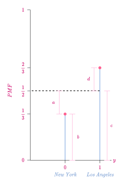
The following diagram is a pictorial representation of the PMFs of X and Y. I have written the place that a particular random value corresponds to for the sake of clarity.
The following diagram illustrates the calculation of total variation distance.
We defined total variation distance as the maximum difference between the probabilities assigned to the same event by two distributions defined on the same sample space.
Looking at the PMFs of X and Y we find that they differ when their random values are either 0 \text{ or } 1 i.e., p_X(0) > p_Y(0) and p_Y(1) > p_X(1).
Let A be the event that either Ann or Kelly in is New York and B be the event that either Ann or Kelly is in Los Angeles. The event B is the same as event A^c since when Ann and Kelly are not in New York they are in Los Angeles.
Total variation distance is the maximum of \big|p_X(A) - p_Y(A)\big| and \big|p_X(A^c) - p_Y(A^c)\big|.
This shows that in order to calculate the total variation distance we find an event in the sample space such that it maximizes the difference between the probabilities assigned to the same event by two distributions. How d0 we find this event?
We choose event A such that the probability of every outcome in event A in one distribution (here p_X) is greater than the probability of the corresponding outcome in event A in the other distribution (p_Y), i.e., p_X(A) > p_Y(A). Since p_X(0) > p_Y(0) (see diagram), so we choose A = \{0\}, namely, the event where either Ann or Kelly is in New York.
Consequently, in the other event A^c = \{1\}, the probability of every outcome in one distribution (p_X) is lesser than or equal to the probability of the corresponding outcome in the other distribution (p_Y), i.e., p_X(A^c) \leq p_Y(A^c).
Since in both the events A \text{ and } A^c, the probabilities of outcomes in one distribution is greater than or equal to the probabilities of outcomes in the other distribution (for A, p_X(A) > p_Y(A) and for A^c, p_Y(A^c) \geq p_X(A^c)), among all the possible subsets of the sample space, these are the only two events that could maximize the difference in probabilities that the two distributions assign to them.
Therefore the total variation distance is either \big|p_X(A) - p_Y(A)\big| \text{ or } \big|p_X(A^c) - p_Y(A^c)\big|. From the figure and our calculation it is seen that \big|p_X(A) - p_Y(A)\big| = \big|p_X(A^c) - p_Y(A^c)\big| = \frac{1}{6}. Is this always the case?
The following is a visual proof for why \big|p_X(A) - p_Y(A)\big| = \big|p_X(A^c) - p_Y(A^c)\big|.
By the axiom of probability,
p_X(A) + p_X(A^c) = 1 = p_Y(A) + p_Y(A^c).
Since A = \{0\} \text{ and } A^c = \{1\},
\begin{equation*}
\begin{split}
p_X(0) + p_X(1) & = p_Y(0) + p_Y(1) \\
\frac{1}{2} + \frac{1}{2} & = \frac{1}{3} + \frac{2}{3} \\
(a + b) + c & = b + (c + d) \\
\text{Cancelling } b + c \text{ from both sides,} \\
a & = d \\
\end{split}
\end{equation*}
Since in order to calculate total variation distance we have to find a particular subset (event), over all possible subsets of the sample space S, that maximizes the difference in probabilities between two distributions and though we found a good way to find this subset, is there a more straightforward way to calculate total variation distance?
We find that the left-hand side of the above equation is just a simple sum over the sample space S i.e., it is the sum of the absolute difference in probabilities that the two distributions assign to each outcome in the sample space. This measure is called the \mathcal{L_1} norm or \mathcal{L_1} distance.
Hence a simple way to calculate total variation distance would be to find the sum of the absolute difference in probabilities that the two distributions assign to each outcome in the sample space and then divide that sum by 2.
In our diagram,
Total Variation Distance = a = d ,
\mathcal{L_1} \text{ norm } = a + d .
Now that we have a sound intuition about total variation distance, in the next part we will give it a mathematically rigorous treatment.
Before we dive into cryptography, we need to understand the concept of distance as a way to distinguish between entities.
In the first part, we will explore how we can use distance to differentiate between entities in a deterministic world. In the next part we will expatiate upon distance as a distinguisher in a probabilistic world. From there on we will proceed to discuss why in cryptography distinguishability between entities (i.e., between two probability distributions or two random variables) matters; and, finally we close the discussion with different ways to measure this distance.
Distance as a Distinguisher in the Real World
John has two identical twin sisters, Ann and Kelly who live in New York and Los Angeles respectively. John has no other siblings. All three of them are my friends.While talking to John I mention that I had met his sister in New York the previous week. John without any doubt (or with 100\% certainty) will know that I’m talking about Ann. Since both Ann and Kelly live in different cities, the distance between them acts as a distinguisher in telling them apart.
Three months later Kelly gets a job as a developer in a tech startup and moves to New York. She lives in Brooklyn while Ann who works as a hedge fund manager in Wall Street, lives in Manhattan. One weekend I bump into Kelly at the MoMA and we have a good time together. Again while talking to John, I mention that I met his sister in New York. Now John is no longer sure which one it is, since both his sisters live in New York. So he can only make a random guess and be 50\% sure which of his sisters I met. Put another way, his advantage in guessing which of his sisters’ I had met has gone down since he is now only 50\% sure compared with his 100\% certainty before. This implies that as the distance between them decreases, their distinguishability also decreases.
Ann is flourishing well at her job and has a fantastic year leaving her with a fat bonus. She moves into 432 Park Avenue on Billionaires’ Row, Manhattan, while Kelly is endlessly grinding away at her job hoping for that IPO event which seems ever more phantasmagorical with each passing year. So one day as an act of resipiscence she quits her job and becomes a social media fashion influencer. She impresses a real estate mogul and she too moves into 432 Park Avenue, though 10 floors higher than self made Ann.
On a lazy Saturday afternoon Ann and I go shopping, commencing at Moschino in Wooster Street, Manhattan. When I meet John for dinner, I recount to him the fabulous afternoon I had with his sister in Manhattan. If he has to guess which sister I’m talking about, even though I’m more specific than the previous occasion (when I just told him that I met one of his sisters in New York), he still has to make a random guess since both now live in the same apartment in Manhattan, separated only by 10 floors. So as the distance between them reduces, they become almost indistinguishable.
So what is the point of this fairy tale like story (those tales generally repeat the same situation thrice 😀)?
The two main takeaways from this story are
The smaller the distance between two entities, the harder it is to tell them apart or distinguish them since you need more information.
When the distance between two entities cannot be sensed by you, then for all practical purposes they are indistinguishable to you. For example, our naked eye cannot distinguish individual stars in the Milky Way because they are so far away and can only see the overall illumination from them. (As we will see later, we will exploit the inability of our computers, due to computational limitations, to distinguish two distributions to build secure systems.)
We humans, for various mostly frivolous reasons, don’t stay put at the same place for the entirety of our lives. So what happens when Ann and Kelly both decide to split their time between New York and Los Angeles? How does the story pan out?
This situation mirrors a move from a deterministic world to a probabilistic one. Our distances will now incorporate probabilistic information and we will see how John fares in this world.
This is a refresher on some basic concepts in probability theory which are often encountered while studying cryptography. We have deliberately tried to keep the discussion simple and hence will not be discussing Sigma Algebra, measurable space, probability measure etc.
Introduction
Since cryptography is about building secure systems, we need a fail proof way to assess an adversary’s chance of breaking the system. We would like to know what is the chance that someone can guess the private key of a bitcoin address, the secret key of a digital signature, decipher an encrypted message etc.
In order to quantify this “chance” in a robust way, we need a logical framework to measure uncertainty and randomness in a systematic way.
Ideally, we design an experiment that models the problem we are trying to solve. This experiment has a set of known outcomes and the likelihood of each of these outcomes occurring is also known. Before the experiment is conducted it is unknown which outcome will occur and hence the uncertainty. One of the possible outcomes gets materialized only after the experiment is performed.
Consider a simple experiment of rolling a fair 6-sided die. This experiment has an outcome of 1, 2, 3, 4, 5 \text{ or } 6. Since each of these outcomes is equally likely, the likelihood of rolling a particular number is \dfrac{1}{6}. Now we can answer some questions like the likelihood of landing a number greater than 4 or less than 3 etc.
The study of probability helps us measure these “likelihoods” in a mathematically precise way.
Definition of Sample Space and Event
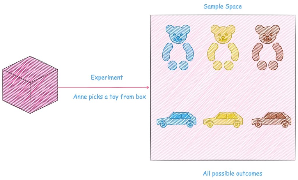
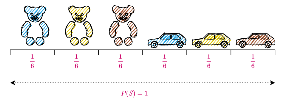
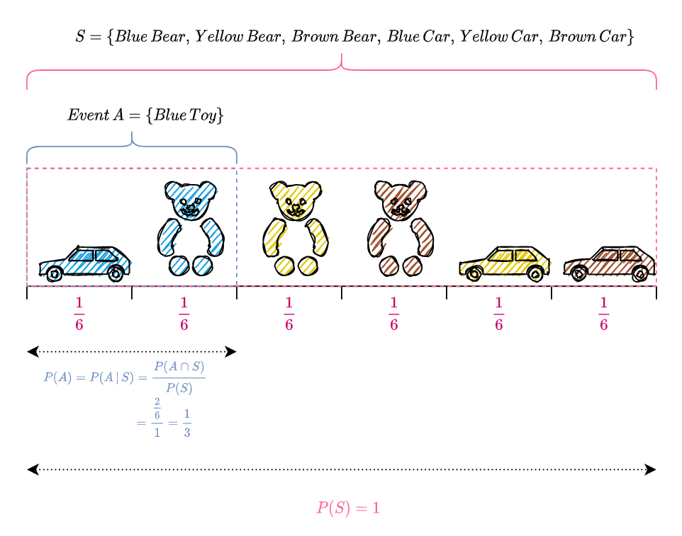
Annie, a little poppet, has a box of toys consisting of 3 bears and 3 cars, in 3 colors namely blue, yellow and brown. Everyday she pulls out a toy at random from the box and plays with it.
What is the likelihood that she will pull out a bear? What is the chance that she plays with a blue toy?
In order to answer these questions, we define an experiment which comprises of Annie pulling out a toy from the box; since she pulls out a toy at random and the toys are arranged such that each toy is equally likely to be picked by her, the outcome of this experiment is equally likely to be any one of the six toys i.e., the likelihood of Annie pulling out a particular toy is \dfrac{1}{6}. Below is a pictorial representation of the experiment and its possible outcomes.
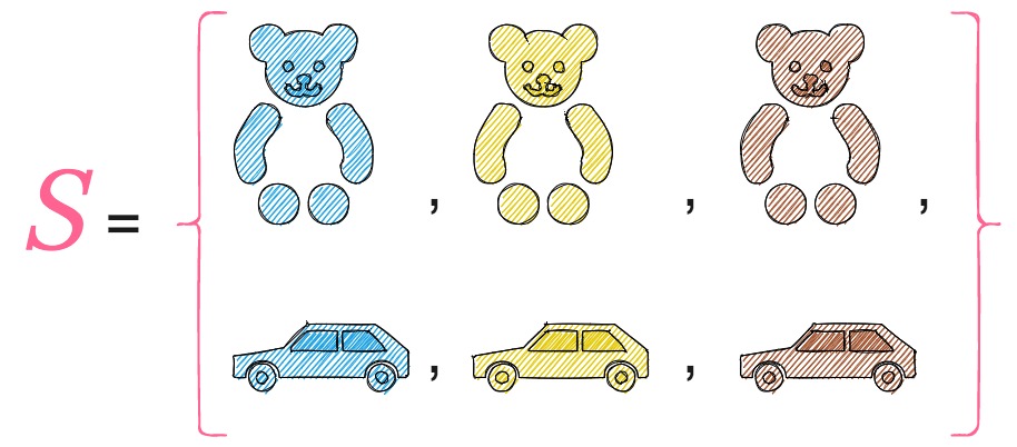
Thesample spaceS of an experiment is the set of all possible outcomes of the experiment. In our case,
Now that we have defined our experiment and the sample space, let us start answering the questions that we posed earlier.
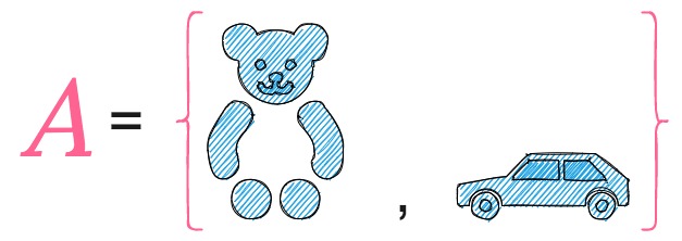
In order to calculate the likelihood of Annie pulling out a blue toy, let us define a subset A, of the sample space S, which comprises of outcomes of the experiment which result in a blue toy i.e.,
The likelihood of A denotes the likelihood of Annie picking a blue toy; this can happen in two ways, when Annie pulls out a blue bear or a blue car. Since the likelihood of pulling out a toy is \dfrac{1}{6}, and the set A has two toys, the likelihood of A is 2 \times \dfrac{1}{6} = \dfrac{1}{3}.
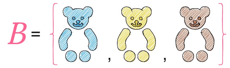
By similar reasoning, to find the likelihood of Annie pulling out a bear, we define a subset B, of the sample space S, which comprises of the outcomes of the experiment which result in a bear i.e.,
The likelihood of B denotes the likelihood of Annie picking a bear; Since the set B has three toys (or three possible outcomes), the likelihood of B is 3 \times \dfrac{1}{6} = \dfrac{1}{2}.
A and B, which are subsets of the sample space S, are called events. When we say that an event A has occurred, we mean that the outcome of the experiment is in A. In this case, the outcome of the experiment is either a blue bear or a blue car.
Cardinality of Sample Space S
The sample space Sof an experiment is called countable if it is finite or countably infinite, otherwise it is called uncountable(also called uncountably infinite).
Countable Set
A set S is countable if :
Its cardinality |S| (the number of elements in the set) is less than or equal to \aleph_0, the cardinality of the set of natural numbers \mathbb{N}, where \mathbb{N} = \{1, 2, 3, \ldots\}.
There exists an injective function (or a one-to-one function i.e., every element of the function’s codomain is the image of at most one element of its domain) \mathcal{f} from S \text{ to } \mathbb{N} i.e., \mathcal{f} : S \rightarrow \mathbb{N}.
S is empty or there exists a surjective function (or onto function i.e., every element of the function’s codomain is the image of at least one element in its domain) \mathcal{f} from \mathbb{N} \text{ to } S i.e., \mathcal{f : \mathbb{N} \rightarrow }S.
There exists a bijective (one-to-one and onto) mapping between S and a subset of \mathbb{N}.
S is either finite(|S| < \aleph_0) or countablyinfinite(|S| = \aleph_0).
All of the above definitions are equivalent.
Finite Set
A set S is finite if there exists a bijection f : \big\{1, 2, \ldots , n\big\} \rightarrow S for some n \in \mathbb{N} (set of all positive integers).
A bijection is a relation between two sets such that each element of either set is paired up with exactly one element of the other set, i.e., a one-to-one correspondence between domain and co-domain.
The number n is the cardinality of set S i.e., |S| = n. The empty set (the unique set having no elements) \{\} \text{ or } \emptyset is considered finite with cardinality zero.
Countably infinite Set
A set S is countably infinite if :
Its cardinality |S| is exactly \aleph_0.
There is an injective and surjective (and therefore bijective) mapping between S \text{ and } \mathbb{N}.
Uncountable Set
A set S is uncountable if :
Its cardinality is neither less or equal to \aleph_0, the cardinality of the set of natural numbers \mathbb{N}.
Its cardinality is strictly greater than \aleph_0 i.e., |S| > \aleph_0.
There exists no injective function from S to \mathbb{N}.
S is nonempty and here exists no surjective function from \mathbb{N} to S.
There exists no bijective mapping between S and \mathbb{N}.
All of the above definitions are equivalent.
Example of a Finite Sample Space
Consider the experiment of tossing two fair coins. The sample space S (possible outcomes) of this experiment is given by, S = \big\{ HH, HT, TH, TT \big\} , where ‘H’ denotes ‘Heads’ and ‘T’ denotes ‘Tails’. Here, n=4 and
f:\{1, 2, 3, 4\} \rightarrow \{HH, HT, TH, TT\}.
The sample space is said to be finite since there is a one to one mapping between the four integers and the outcomes of the sample space.
Example of a Countably Infinite Sample Space
Let us consider the experiment of tossing a fair coin till a head appears. The sample space S of this experiment is given by, S = \big\{ H, TH, TTH, TTTH, \ldots \big\} , where ‘H’ denotes ‘Heads’ and ‘T’ denotes ‘Tails’. Every positive integer can be mapped to an element in the sample space as shown below.
Since there exists a bijective mapping between S and \mathbb{N}, the set of all positive integers, S is countably infinite.
Example of an Uncountable Sample Space
Suppose we conduct an experiment measuring the weight of a man in kilograms on a particular day. The sample space S is the set of all positive real numbers in the interval \big[45, 250\big] i.e., S = \big\{ s \in \mathbb{R}\, |\, 45 \leq s \leq 250 \big\}. We can use Cantor’s diagonal argument to prove that this set is uncountable because for any list of numbers in the interval \big[45, 250\big], there will always be numbers in \big[45, 250\big] that are not on the list.
For example, suppose we construct a list of numbers between \big[45, 250\big] as \big[45, 45.5, 46, 46.5, \ldots, 250\big], we can always construct another list \big[45, 45.1, 45.2, \ldots, 46.1, 46.2, \ldots, 250\big] that has numbers not included in the previous list.
Also if an uncountable set X is a subset of a set Y, then Y is uncountable as well. Since we have shown that the set of all positive real numbers in the interval \big[45, 250\big] is uncountable, it follows that the set \mathbb{R} of all real numbers is uncountable as well.
Equivalently, the set S is uncountable or uncountably infinite since there is no bijective mapping between S and the set of all positive integers, \mathbb{N}. Also, the cardinality of set S is strictly greater than \aleph_0, the cardinality of the set of all positive integers.
Definition of Discrete Sample Space
A sample space S is called discrete if S is countable i.e., S is finite or countably infinite.
Definition of Continuous Sample Space
A sample space S is called continuous if S is uncountable.
Definition of Probability
A probability space consists of a sample space S and a probability function P which takes an event A\subseteq S as input and returns P(A), a real number between 0 and 1, as output.
P(A) is the mathematical term for the “likelihood of A” that we had discussed previously.
The function P must satisfy the following axioms:
P(\emptyset) = 0, \, P(S) = 1
If A_1, \, A_2, \, \ldots are disjoint events, then
P \Big(\underset{j\,=\,1}{\overset{\infty}{\cup}}A_j\Big) = \underset{j \,= \, 1}{\overset{\infty}{\sum}}\, P(A_j).
Disjoint events means that the events are mutually exclusive : A_i \cap A_j = \emptyset for i \neq j.
Note:
\emptyset denotes an empty set i.e., a set with no elements in it.
Union of n events A_1, \ldots, A_n, denoted by A_1 \cup A_2 \cdots \cup A_n, is the occurrence of at least one of the events A_1, \ldots, A_n.
Intersection of two events A \text{ and } B, denoted by A \cap B, is the simultaneous occurrence of both the events A \text{ and } B. Similarly, for n events, A_1 \cap A_2 \ldots \cap A_n, denotes the simultaneous occurrence of all the n events.
Let us represent these axioms pictorially, in the context of the experiment in which Annie picks up a toy at random from a box.
Since the sample space S represents all possible outcomes of the experiment,
The pictorial representation of each outcome of the sample space S is shown on top of a line segment, whose length equals the probability of that particular outcome occurring. Since, as per the first axiom, P(S) = 1, the summation of the lengths of all the line segments, where each segment’s length represents the probability of a particular outcome occurring, equals 1.
To illustrate the second axiom, let us define define two events,
A_1 = \{Blue\, Bear\} and A_2 = \{Blue\, Car, Yellow\, Car, Brown\, Car\}, where A_1 denotes the event that occurs when Annie picks a blue bear and A_2 denotes the event that occurs when Annie picks a car.
Since a toy cannot be both a bear and a car, A_1 and A_2 are disjoint events, i.e., A_1 \cap A_2 = \emptyset.
Let us calculate the probabilities of each of the events A_1 and A_2 occurring.
Annie can pick a car in three ways i.e., she can pick a car by either picking a blue, yellow or brown car. Hence the event A_2 can occur in three possible ways and so comprises of three possible outcomes. Since the probability of each outcome is \dfrac{1}{6}, the total probability of the entire event A_2 is
Let us calculate the probability of Annie picking either a blue bear or a car i.e., the probability of event A_1 or A_2 occurring, which is denoted by, P(A_1 \cup A_2).
The second axiom is graphically represented below.
Conditional Probability
Let us develop some intuition for conditional probability by revisiting the experiment in which little poppet Annie picks a toy from her box.
The sample space S of the experiment together with the events A \text{ and } B are pictorially represented below.
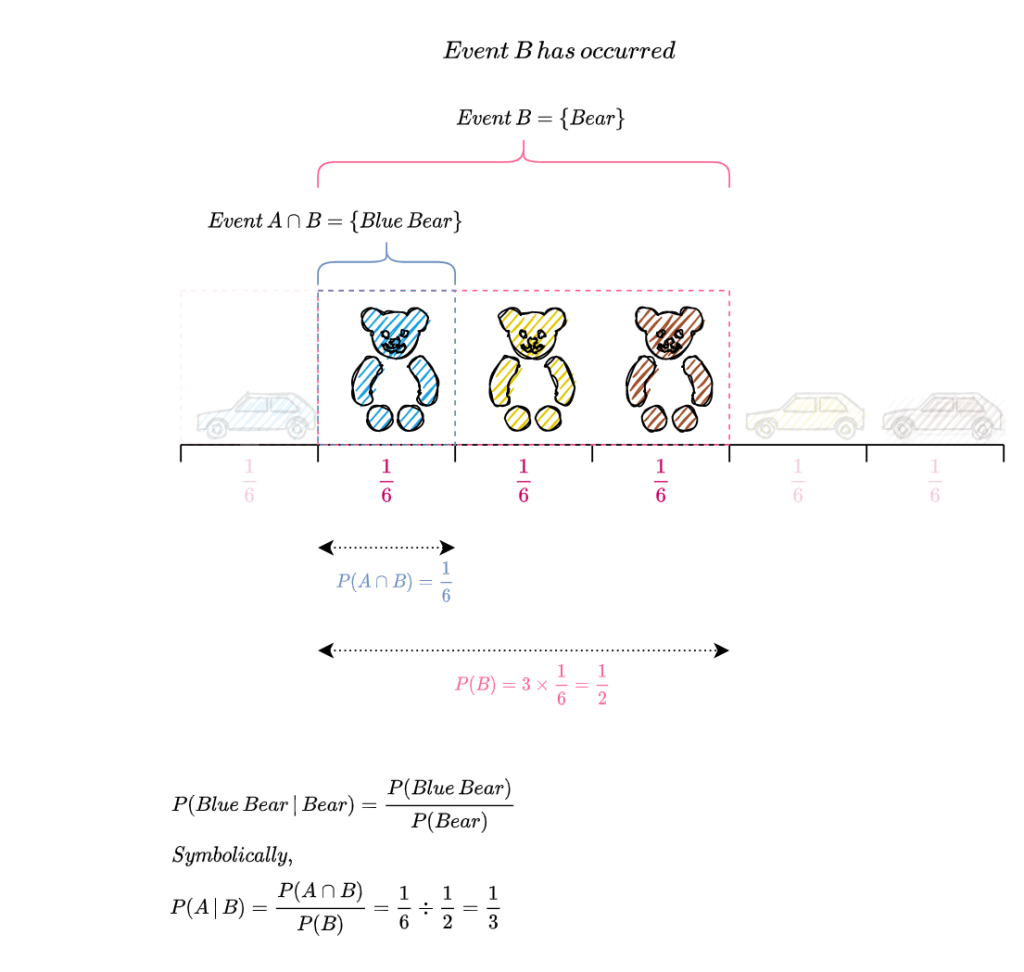
Suppose we get to know that Annie has picked a bear, what is the probability that it is a blue bear? Reframing this question in the probabilistic framework, what is the probability of event A (Annie picks a blue toy) occurring, given that event B(Annie picks a bear), has occurred? This is represented symbolically as P(A\,|\,B).
Since we know that Annie picked a bear i.e., event B occurred, we get rid of all the outcomes in B^c (the set of elements not in B), since it is incompatible with the knowledge that B occurred. All the outcomes in B^c are greyed out in the figure below. From the figure we can see that there is only one outcome remaining in A and its probability is given by P(A \cap B) = \frac{1}{6}. So the probability that Annie picked a blue bear i.e.,
The calculation of P(A\,|\, B) is pictorially represented below.
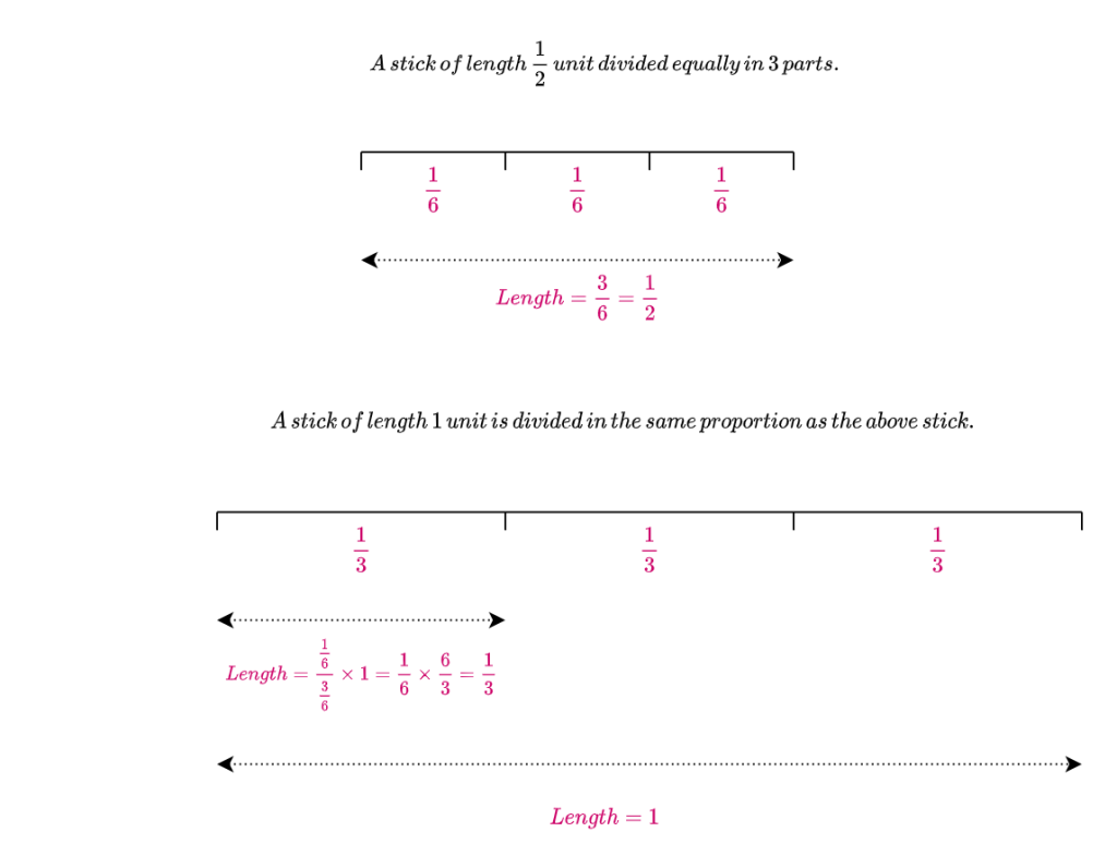
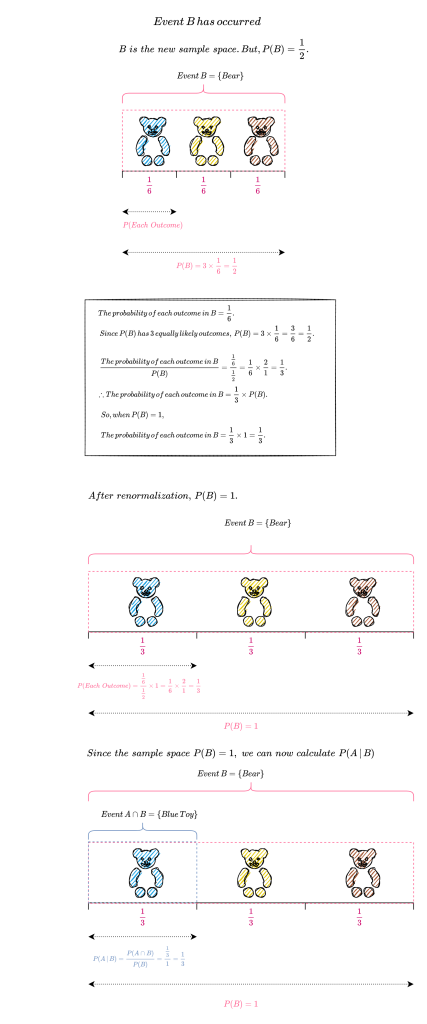
Since B has occurred, we must calculate the probability of all outcomes with respect to B. So B becomes the new sample space and as per the first axiom of probability, P(B) must equal 1. From the above diagram, we can see that P(B) = \frac{1}{2}. So we need to renormalize P(B) so that it sums to 1 while keeping the proportion of the probability of each outcome in B with respect to the probability of B the same. How do we do this?
The figure below illustrates how to increase the length of a stick from \frac{1}{2} unit to 1 unit while maintaining the proportion of its individual divisions.
The figure below shows the renormalization of P(B) so that it sums to 1.
Why is P(A\,|\,B) = \frac{1}{3} irrespective of whether P(B) = \frac{1}{2} or P(B) = 1 ? Since P(A\,|\,B) is the ratio between P(A \cap B) and P(B), this ratio does not change when P(B) is proportionally scaled.
Let us consider a more mundane example to illustrate this point. Suppose George weighs 50 kgs and Jamie weighs 100 kgs, the ratio of the weight of George to Jamie is \frac{50}{100} = \frac{1}{2}. Now suppose instead of kgs we measure their weight in pounds, the ratio of their weights would still remain the same i.e., Jamie’s weight will still be double of George’s. Lets verify this by calculation. Since 1 kg = 2.20462 pounds, the ratio of their weights is \frac{50 \times 2.20462}{100 \times 2.20462} = \frac{1}{2}.
In our case, when P(B) = \frac{1}{2}, P(A\,|\,B) = \frac{\frac{1}{6}}{\frac{1}{2}} = \frac{1}{3} and when P(B) = 1, P(A\,|\,B) = \frac{\frac{1}{6} \times 2}{\frac{1}{2} \times 2} = \frac{\frac{1}{6}}{\frac{1}{2}} = \frac{1}{3}.
From this discussion on conditional probability, it is obvious that whenever we calculate the probability of an outcome or an event it is always with respect to a sample space. So when we calculated P(A) i.e.,the probability of Anne picking a blue toy we actually calculated P(A \,|\, S). This is illustrated in the figure below.
It should be noted that conditional probabilities are still probabilities and so they must satisfy the axioms of probability.
Definition of Conditional Probability
If A \text{ and } B are events in a sample space S, with P(B) > 0, then the conditional probability of A given B, denoted by P (A\,|\,B) , is defined as,
P(A\, |\,B) = \frac{P(A\cap B)}{P(B)}
P(A\,|\,B) is the probability of an event A occurring, given that the event B has occurred i.e., we want to update the probability of event A occurring in light of the new evidence that event B has occurred. We call P(A) the prior probability of A and P(A\,|\,B) the posterior probability of A (“prior” means before updating based on the evidence, and “posterior” means after updating based on the evidence).
Probability of the Intersection of Two Events
For any events A \text{ and } B with positive probabilities,
P(A \cap B) = P(B)\, P(A \,|\, B) = P(A)\, P(B \,|\,A).
This follows from taking the definition of conditional probability i.e., P(A\,|\,B) = \dfrac{P(A \,\cap\, B)}{P(B)} and multiplying both sides by P(B), to get P(A \cap B) = P(B)\, P(A \,|\, B).
Similarly by taking the definition of conditional probablility as P(B\,|\,A) = \dfrac{P(A \,\cap\, B)}{P(A)}and multiplying both sides by P(A) we get P(A \cap B) = P(A)\, P(B \,|\, A).
From the definition of conditional probability, P(A\,|\,B) = \dfrac{P(A \,\cap\, B)}{P(B)} and the probability of the intersection of two events, P(A \cap B) = P(A)\, P(B \,|\, A), it follows that,
P(A\,|\,B) = \frac{P(A)\, P(B \,|\,A)}{P(B)}.
This result which relates P(A\,|\,B) to P(B\,|\,A) is called Bayes’ Theorem.
Independence of Events
When events provide no information about each other, they are said be to independent.
Independence of Two Events
Events A \text{ and } B are independent if and only if P(A\cap B) = P(A) P(B).
Let us assume that A and B are independent events i.e., P(A\cap B) = P(A) P(B), with P(A) > 0 and P(B) > 0.
Intuitively, if A \text{ and } B are independent, then learning that B has occurred provides us with no information whether or not A has occurred (and vice versa).
Random Variable
Definition
Given an experiment with sample space S, a random variable X is a function that maps the sample space S to the real numbers \mathbb{R} i.e., X: S \rightarrow \mathbb{R}.
By convention, a random variable is usually denoted by capital letters X, Y, Z and its values by lower case letters x, y, z.
A random variable X assigns a numerical value X(s) to each possible outcome s of the experiment. Each outcome of the experiment could be mapped to the same numerical value.
The random variable X is a numerical summary of some aspect of the experiment.
The source of randomness for X is the experiment itself, in which a sample outcome s \in S is chosen according to a probability function P. Before we perform the experiment, the outcome s has not yet been realized, so we don’t know the value of X. Once the experiment is completed and the outcome s is known, X crystallizes into the numerical value X(s).
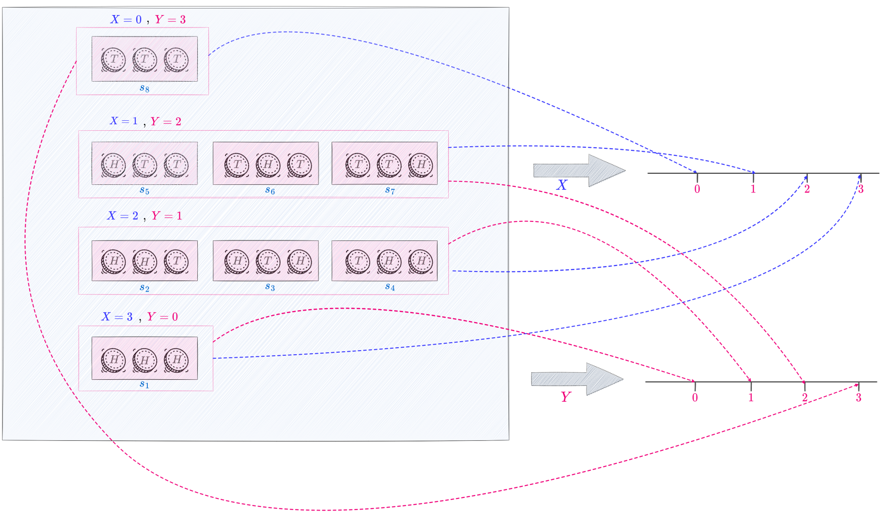
As an example, consider an experiment where we toss a fair coin thrice. The sample space consists of eight possible outcomes : S = \{ HHH, HHT, HTH, THH, HTT, THT, TTH, TTT \}.
Let X be the number of heads. This is a random variable with 0, 1, 2 and 3 as possible values. In terms of the function notation, X assigns the value 0 to the outcome TTT, 1 to the outcomes HTT, THT \text{ and } TTH, 2 to the outcomes HHT, HTH \text{ and } THH and 3 to the outcome HHH. That is,
X (TTT) = 0
X (HTT) = X (THT) = X (TTH) = 1
X ( HHT) = X (HTH) = X (THH) = 2
X (HHH) = 3
We can define any number of random variables on the same sample space, each numerically summarizing a different aspect of an experiment.
Let Y be the number of tails. Since X + Y = 3 , in terms of X, we have Y = 3 - X.
Y(s) = 3 - X(s)
In the above example X and Y are two random variables defined on the same sample space though X denotes the number of heads and Y the number of tails that result when a fair coin is tossed thrice.
The following figure graphically represents the mapping of the sample space S to the real line by the random variable X, which denotes the number of heads and the random variable Y, which denotes the number of tails that result in an experiment where we toss a fair coin thrice. The random variables, X and Y, are defined on the same sample space S, though they summarize different aspects of the experiment. While random variable X maps the outcome s_1, namely, that of the three tosses of the fair coin resulting in heads, to 3, the random variable Y maps the same outcome s_1 to 0, since it represents the number of tails that occur in three tosses of a fair coin.
Types of Random Variable
There are two main types of random variables, namely, discrete random variables and continuous random variables.
Discrete Random Variable
A discrete random variable X is a function that maps a discrete sample space S (this means S is countable i.e., either finite or countably infinite) to the real numbers \mathbb{R}. Specifically, to each element s\in S, we assign the real number X(s). So the possible values of a discrete random variable form a countable set.
If X is a discrete random variable, then the finite or countably infinite set of values x such that P(X = x) > 0 is called the support of X. Usually in applications, the support of a discrete random variable is a set of positive integers.
Examples of Discrete Random Variable
Following are some examples of discrete random variables :
The number of applicants for a job.
The number of girls in a randomly selected two-child family.
The number of heads in two tosses of a coin.
The number of customers arriving at a bookstore between 7:00 p.m. and 9:00 p.m.
Continuous Random Variable
A continuous random variable can take any real value in an interval and its possible values form an uncountably infinite set.
Examples of Continuous Random Variable
Following are some examples of continuous random variables :
The weight of refuse on a truck arriving at a landfill.
The temperature of a cup of tea served at a restaurant.
The air pressure of a tire on an automobile.
The amount of rain recorded at an airport one day.
Note on random variables used in cryptography: Since in cryptography we mostly deal with finite sample spaces for example message space, key space etc we use discrete random variables to a large part. Hence the following discussion will pertain only to discrete random variables.
Distribution of a Discrete Random Variable
The distribution of a random variable specifies the probabilities of all events associated with the random variable. Say, for the random variable X denoting the number of girls in a randomly selected two-child family, the distribution enumerates the probability of X equaling 0, 1 \text{ or } 2. Using this distribution, we can calculate the probability that there is at least one girl child. The distribution helps us in answering questions about the probability that a random variable will fall within a given range or be greater or less than a particular value etc.
In our example, each of these numbers in the support of X namely 0, 1 \text{ or } 2 corresponds to an event in the sample spaceS = \{ GG, GB,BG, BB \} of equally likely outcomes. (‘G’ denotes a girl and ‘B‘ a boy). \{ X = 1 \} consists of the sample outcomes GB and BG which are the two outcomes to which X assigns the number 1. Since \{ GB, BG \} is a subset of the sample space, it is an event. Similarly, \{ X = 0 \} consists of the only sample outcome \{ BB \} to which X assigns the number 0 and \{ X = 2 \} consists of the only sample outcome \{ GG \} to which X assigns the value 2. The probability \{ X = 0 \} \text{ is } \frac{1}{4} (each outcome in the sample space is equally likely and there is only one outcome corresponding to this event.) Similarly, probability \{ X = 1 \} \text{ is } \frac{2}{4} = \frac{1}{2} and \{ X = 2 \} \text{ is } \frac{1}{4} . The probability that there is at least one girl child is the event \{X \geq 1\} i.e., X = 1 or X = 2 which is \frac{1}{2} + \frac{1}{4} = \frac{3}{4} (when two events are disjoint we add their probabilities).
Now that we have an understanding of the distribution of a discrete random variable, let us define it in a mathematical way.
For a discrete random variable, the most intuitive way to express its distribution is with a probability mass function.
Definition
Let X be a discrete random variable and let x_1, x_2, \ldots be the values which it assumes. The aggregate of all the outcomes s of the sample space S to which X assigns the number x_j forms the event X = x_j. This event is also written as \{X = x_j\}; formally, \{ X = x_j\} is defined as \{s \in S : X(s) = x_j\}, but writing \{ X = x_j\} is shorter and more intuitive. Its probability is denoted by P(X = x_j). The probability mass function (PMF) of a discrete random variable X is defined as the function p_X such that p_X(x_j) = P(X = x_j).
Clearly, p_X(x_j) \geq 0 (positive if x_j is in the support of X , 0 otherwise) and \Sigma \, p_X(x_j) = 1.
Let us construct the probability mass function of the random variable X denoting the number of girls in a randomly selected two-child family.
Since X equals 0 if BB occurs, 1 if GB or BG occurs, and 2 if GG occurs, the PMF of X is the function p_X given by,
p_X(0) = P(X = 0) = \frac{1}{4},
p_X(1) = P(X = 1) = \frac{1}{2},
p_X(2) = P(X = 2) = \frac{1}{4},
and p_X(x) = 0 for all the other values of x.
Functions of Random Variables
What does it mean to take a function of a random variable? A function g(X) of a random variable X is any function g that maps real numbers to real numbers i.e., g : \mathbb{R} \rightarrow \mathbb{R}.
A function of a random variable is also a random variable with its source of randomness being the experiment. We know that a random variable maps each outcome of an experiment s in the sample space S to a real number. Let X be a random variable defined on a sample space S with 6 outcomes namely s_1, s_2, \ldots, s_6. If we apply the function g to the numbers X(s_1) through X(s_6), we now have numbers g(X(s_1)) through g(X(s_6)) , which gives a new mapping from sample outcomes to real numbers and we have essentially created a new random variable, g(X) .
Thus if X is a random variable, then X^2, e^X and cos(X) are also random variables.
Suppose X is a random variable that denotes the number of heads that turn up when a fair coin is tossed thrice. Then g(X) = 3 - X is the number of tails resulting from three tosses of the coin. Since X is a random variable, g(X) is also a random variable; both deriving their source of randomness from the experiment of tossing the coin thrice whose outcome is unknown until the experiment is conducted.
Definition of Function of a Random Variable
For an experiment with sample space S, a random variable X, and a function g : \mathbb{R} \rightarrow \mathbb{R}, g(X) is the random variable that maps s to g(X(s)) for all s \in S.
Suppose g(X) = X^2, the figure below shows that g(X) is the composition of the functions X and g. If X crystallizes to 3, then g(X) crystallizes to 9.
The random variable X is defined on a sample space S with 8 outcomes, and has possible values 0, 1, 2 \text{ and } 3. The function g is the square function. Composing X and g gives the random variable g(X) = X^2, which has possible values 0, 1, 4 \text{ and } 9.
Independence of Random Variables
Intuitively, if two random variables X and Y are independent, then knowing the value of X gives us no information about the value of Y and vice versa.
Definition
Independence of Two Random Variables
Random variables X and Y are said to be independent if,
P(X \leq x, Y \leq y) = P(X \leq x)P(Y \leq y), \,\forall\, x, y \in \mathbb{R}.
In the discrete case this is equivalent to the condition,
P(X = x, Y = y) = P(X = x)P(Y = y), \,\forall\, x \in X\, \text{and}\, y \in Y.
Independence of Many Random Variables
Random variables X_1, \ldots, X_n are independent if,
P ( X_1 \leq x_1, \ldots, X_n \leq x_n ) = P ( X_1 \leq x_1 ) \ldots P (X_n \leq x_n), \forall x_1, \ldots , x_n \!\! \in \mathbb{R}.
For infinitely many random variables, we say that they are independent if every finite subset of the random variables is independent.
Functions of Independent Random Variables
If X and Y are independent random variables, then any function of X is independent of any function of Y .
Conditional Independence of Random Variables
Random variables X and Y are conditionally independent given another random variable Z if for all x, y \epsilon \, \mathbb{R} and all z \in Z,
P(X \leq x, Y \leq y \,|\, Z = z) = P(X \leq x \,|\, Z = z)\, P(Y \leq y \,|\, Z = z).
For discrete random variables, the equivalent condition is
P(X = x, Y = y \,|\, Z = z) = P(X = x \,|\, Z = z)\,P(Y = y \,|\, Z = z).
Conditional Probability Mass Function
For any discrete random variables X and Y , the function P (X = x \,|\, Y = y) , when considered as a function of x for fixed y, is called the conditional probability mass function of X given Y = y .
Expectation
Intuitively, the expected value of a random variable can be thought of as the average of values attained by the random variable in repeated trials of the experiment.
Consider the experiment of tossing a fair coin twice. Let X be the number of heads. We perform this experiment n times, where n is a very large number, and note down the value realized by X each time. If we take the arithmetic mean of all the numbers observed (add all the numbers and divide by n), then by the law of large numbers, this mean will be very close to the expectationE(X) of the random variable X.
If each outcome is not equally likely, then the arithmetic mean becomes the weighted mean, where each outcome is weighted by its probability of occurring.
Definition
Let X be a discrete random variable assuming the values x_1, x_2, \ldots with corresponding probabilities p_X(x_1), p_X(x_2), \ldots . The expectation (also called expected value or mean) of X is defined by
E(X) = \sum_{n=1}^{\infty} x_{n}\ p_{X}(x_n)
provided that the series converges absolutely. In this case we say that X has a finite expectation. If \sum_{n=1}^{\infty} \ \lvert x_n \rvert \ p_X(x_n) diverges, then X has no finite expectation i.e., the expectation of X is undefined. This is because either the series E(X) diverges or its value depends on the order in which the x_ns are listed.
The expected value of a discrete random variable is a weighted average of the possible values that the random variable can take on, weighted by their probabilities.
If anyone is wondering why we are interested in the convergence or divergence of \sum_{n=1}^{\infty} \ \lvert x_n \rvert \ p_X(x_n), let us take a little detour to calculus to answer this question.
Calculus Refresher :
A series \sum_{n=1}^{\infty}a_n is absolutely convergent if the series of absolute values \sum_{n=1}^{\infty}\ \lvert a_n\rvert is convergent.
If a series \sum_{n=1}^{\infty}a_n is absolutely convergent, then it is convergent (the series sums to a single value as n \rightarrow \infty).
A series \sum_{n=1}^{\infty}a_n is conditionally convergent if it is convergent but not absolutely convergent, i.e., if \sum_{n=1}^{\infty}a_n converges but \sum_{n=1}^{\infty}\ \lvert a_n\rvert diverges (the series does not sum to a single value as n \rightarrow \infty).
It is important to know whether a given convergent series is absolutely convergent or conditionally convergent because this determines whether infinite sums behave like finite sums.
Even if we rearrange the order of terms in a finite sum, the value of the sum remains unchanged. But this is not always the case for an infinite series.
By a rearrangement (or permutation) of an infinite series \sum_{n=1}^{\infty}a_n we mean a series obtained by simply changing the order of the terms.
For example, one permutation of \sum_{n=1}^{\infty}a_n , could start as follows:
It can be proved that if \sum_{n=1}^{\infty}a_n is an absolutely convergent series with sum s, then any rearrangement of \sum_{n=1}^{\infty}a_n has the same sum s.
However, any conditionally convergent series can be rearranged such that the new series either converges to an arbitrary real number or even diverges.
This was proved by Reimann and following is the statement of Riemann’s Rearrangement Theorem:
Let \sum_{n=1}^{\infty}a_n be a conditionally convergent series of real terms, and let S be a given real number. Then there is a rearrangement \sum_{n=1}^{\infty}b_n of \sum_{n=1}^{\infty}a_n such that \sum_{n=1}^{\infty}b_n = S. There also exists a rearrangement \sum_{n=1}^{\infty}b_n such that \sum_{n=1}^{\infty}b_n = \infty . The sum can also be rearranged to diverge to -\infty or to fail to approach any limit, finite or infinite.
Note: I have not proved any of these results. Sometime in the future (when time permits) I might write a detailed note on Sequences and Series with proof of these statements. If you want to go deeper you can refer either to Tom Apostol’s Calculus Volume 1 or for fun and challenge try to prove them yourself. 🙂
Now coming back to our series, E(X) = \sum_{n=1}^{\infty} x_{n}\ p_{X}(x_n), we have three cases :
The series \sum_{n=1}^{\infty} x_n \ p_X(x_n)diverges. In this case, the expectation E(X) does not exist and is undefined.
The series \sum_{n=1}^{\infty} x_n \ p_X(x_n) is absolutely convergent (i.e.,\sum_{n=1}^{\infty} \ \lvert x_n \rvert \ p_X(x_n) is convergent). This implies that the expectation E(X) converges and any rearrangement of \sum_{n=1}^{\infty} x_n \ p_X(x_n) has the same sum. So the expectation E(X) exists and is finite.
The series \sum_{n=1}^{\infty} x_n \ p_X(x_n) is conditionally convergent (i.e., \sum_{n=1}^{\infty} x_n \ p_X(x_n) converges but \sum_{n=1}^{\infty} \ \lvert x_n \rvert \ p_X(x_n) diverges). This implies that terms in the series could be rearranged such that E(X) could either converge to an arbitrary real number or even diverge. Hence the expectation E(X) is undefined.
Some Examples of Expectation Calculation
Expectation of a roll of a fair die
Let X be a discrete random variable that denotes the result of rolling a fair 6-sided die. X can take on any of the values 1, 2, 3, 4, 5, 6 with equal probabilities of \frac{1}{6} . Using the definition, the expected value,
It should be noted that the expected value is not one of the possible outcomes; its obvious that we cannot roll a 3.5. 😉 However, if we average the outcomes of a large number of rolls, the result approaches 3.5.
Expectation of profit from the purchase of a raffle ticket
Let us look at an interesting use case. Suppose your city organizes a raffle once a month. A thousand tickets are sold for \$1 each. Each ticket has an equal probability of winning. There are three prizes to be won; namely the first price is \$300, the second prize is \$200 and the third prize is \$100. Sam would like to participate in this monthly raffle. He has two questions he wants to know the answers to which will help him decide whether it is profitable for him to participate in this raffle; namely
What is the probability of winning any money on the purchase of one ticket?
If Sam were to participate in this raffle every month, on average how much does he expect to win (or lose)?
With our knowledge of probability let us help him answer these questions. We model this problem by first coming up with a random variable that denotes the profit on the purchase of one ticket and then constructing a probability distribution that assigns specific probabilities to each of the value that random variable can take. We can then answer the questions using the probability distribution of the random variable.
Let X be the discrete random variable that denotes the profit from the purchase of one raffle ticket. X can take any of the values 299, 199, 99, -1 (since \$1 was paid to purchase the ticket, this amount was subtracted from the winnings). The probability distribution of X is given by,
This means that if Sam were to play the raffle repeatedly, then although he might win sporadically, on average he would lose 40 cents per ticket purchased.
Linearity of Expectation
If Xand Y are random variables with finite expectations, then the expectation of their sum exists and is the sum of their expectations:
E(X + Y) = E(X) + E(Y)
The random variables X and Y are functions that assign a real number to every outcome s in the sample space. They may also assign the same value to multiple sample outcomes.
If X(s) is the value that X assigns to the outcome s, then
E(X) = \sum_sX(s) \ P\big(\{s\}\big)
where P\big(\{s\}\big) is the probability of the outcome s occurring.
Similarly for random variable Y defined on the same sample space S,
Since X and Y have finite expectations, we know that the series E(X) and E(Y) converge absolutely. So the sum can therefore be rearranged (since an absolutely convergent series sums to the same value even when its terms are rearranged) to \sum_s\big(X(s) + Y(s)\big) \ P\big({s}\big) which by definition is the expectation of X+Y. This proves that E(X+Y) exists.
Note: If f \text{ and } g are two functions, then (f+g)(x) := f(x) + g(x) . The domain of (f+g) is the intersection of the domains of f and g and the range the union of their respective ranges.
The linearity of expectation is true for any number of random variables. If X_1, X_2, \ldots, X_n are random variables numerically summarizing different aspects of a certain experiment, then,
E(X_1 + \dots + X_n) = E(X_1) + \cdots + E(X_n).
Joint Distribution
Individual distributions of two random variables do not provide any information about whether the random variables are independent or dependent. For example, random variables X \text{ and } Y are independent if they indicate Heads on two different coin flips and dependent if they indicate Heads and Tails on two different coin flips. (If X indicates Heads, then Y = 2 - X indicates Tails.) Joint distributions capture information about how multiple random variables interact. Suppose we want to study how stock prices evolve over time, and since there could be a multitude of factors affecting prices and these factors could be interrelated it would be better to study these factors in tandem than in isolation and the joint distribution provides us with a framework for doing this.
The distribution of a single random variable X provides complete information about the probability of X falling into any subset of the real line. Analogously, the jointdistribution of two random variables X and Y provides complete information about the probability of the vector (X, Y) falling into any subset of the plane.
As already discussed, since in cryptography we work only with discrete random variables, we will only discuss the joint distribution of discrete random variables.
Definition
Consider two discrete random variables X \text{ and } Y defined on the same sample space S. Let x_1, x_2, \ldots \text{ and } y_1, y_2, \ldots denote the values which they assume, respectively. Also, let the corresponding probability distributions of X \text{ and } Y be p_X(x_i) \text{ and } p_Y(y_j) for i, j = 1, 2, \ldots.
The aggregate of outcomes (of the experiment) in the sample space S for which the two conditions X = x_i \text{ and } Y = y_j are satisfied forms an event (X = x_i, Y = y_j), whose probability is denoted by P(X = x_i, Y = y_j). The function
p_{X, Y}(x_i, y_j) = P(X = x_i, Y = y_j)
is called the joint probability distribution (or joint PMF) of X \text{ and } Y.
Like the PMFs of single random variables, the joint PMFs must also be nonnegative and sum to \mathcal{1}, where the sum is taken over all possible values of X \text{ and } Y i.e.,
The joint PMF of n discrete random variables is defined analogously.
Since the joint PMF describes the probability distribution of (X, Y), we can use it to find the probability of the event (X, Y) \in A, where A is the set of points in the support of (X, Y), by simply summing the joint PMF over A i.e.,
The joint distribution encodes the marginal distributions i.e., the distributions of each of the individual random variables.
The marginal distribution of X is the probability distribution of X wherein the probability of each value of X is obtained by summing the joint distribution of the random variables X \text{ and } Y over all values of Y corresponding to that particular value of X.
Definition
For discrete random variables X \text{ and } Y, the marginalPMF of X is
The operation of summing over all the possible values of Y in order to convert the joint PMF of X \text{ and } Y into the marginal PMF of X is known as marginalizingoutY.
The joint distribution also encodes the conditional probability distributions, which describes the probability distribution of a random variable based on the realized values of other random variables.
Suppose we observe the value of X and want to update the distribution of Y to incorporate this information. Since the marginal PMF, P(Y = y), does not incorporate any information about X, we should use a PMF that conditions on the event X = x, where x is the value observed for X. We call this PMF the conditional PMF.
Definition
The conditional distribution (or conditional PMF) of Y given X = x is the updated distribution for Y after observing X = x.
For discrete random variables X \text{ and } Y , the Bayes’ rule relates the conditional probability distribution of Y given X = x to that of X given Y = y as follows:
P (Y = y \,|\, X=x ) = \frac{P(Y=y,X=x)}{P(X=x)} = \frac{P(Y=y) P(X=x \,|\, Y=y)}{P(X=x)}\cdot
This is viewed as a function of y for a fixed x .
The conditional distribution gives us an alternate way to calculate the marginal distribution.
Discrete random variables X \text{ and } Y are independent if for allx \text{ and } y ,
P(X = x, Y = y) = P(X = x)P(Y = y).
When two discrete random variables are independent, their individual distributions (or marginal distributions) are all we need in order to construct their joint distribution; we can get the joint PMF by multiplying the marginal PMFs. In general the marginal distributions do notdetermine the joint distributions; otherwise there would be no need for joint distributions.
The independence is also equivalent to the condition
P(Y = y \,|\, X = x) = P(Y = y)
for all x, y such that P(X = x) > 0.
This is because for all x, y such that P(X = x) > 0,
P(Y = y \,|\, X = x) = \frac{P(Y=y,X=x)}{P(X=x)} = \frac{P(X=x) P(Y=y)}{P(X=x)} = P ( Y = y ).
The above equation shows that when two random variables are independent, all the conditional PMFs are the same as the marginal PMFs.