The Story of Total Variation Distance.
You can read Part 1 of the story here.
Ann’s hedge fund decides to invest in movies and Ann has to move to Los Angeles for 6 months to meet with Hollywood production houses and make deals. Meanwhile Kelly is growing immensely successful as a fashion influencer and has been offered a role in the documentary “The Lives of Famous Wenches”. She would be shooting in Los Angeles for 8 months.
Ann is in New York from January to June and for the remaining 6 months (July to December) she is in Los Angeles. Kelly is in New York from January to April and for the remaining 8 months (May to December) she is in Los Angeles.
The following table pictorially represents their whereabouts throughout the year.

As Kelly’s fame grows, she is getting noticed by an underworld criminal network, who wants to kidnap her for ransom. Meanwhile Michael, an out of work hitman (in this era of cancel culture why would a person need to be murdered to be done away with, when all that is required is to assassinate his character), feeling maudlin with self pity, is hired for the job. The underworld don contacts Michael and asks him to kidnap Kelly, providing him with a photo of Kelly and also information about when Kelly would be in New York and when she would be in Los Angles. The don is however unaware of Kelly’s identical twin sister, Ann, and hence Michael is also ignorant of Ann’s existence. Also Michael will kidnap Kelly at the most opportune time when he is sure that he would not be caught by the police.
Since Michael runs some risk of getting caught by the police, he wants to know whether he has an advantage in this kidnapping game. Does he succeed with a higher probability than if he had just succeeded at random?
Before answering these questions, let us take a little detour to understand some important concepts like bias and advantage with an intuitive example. We will then connect these concepts to the story of statistical distance.
Note: It is of paramount importance to understand bias and advantage as they form the basis of many security proofs in cryptography. If you are already familiar with these concepts you can continue reading, though I would still prefer that the reader peruses the example so that we are on the same page.
Now that we are familiar with advantage and bias, let us use these concepts to answer whether Michael has an advantage with respect to Kelly. We can view the kidnapping as a game with two participants, namely, Michael and Kelly. If Michael wins the game it means that he successfully kidnaps Kelly and hence he wins and Kelly loses. On the contrary, if Michael loses it means that he fails to kidnap Kelly and hence Kelly wins.
\begin{equation*}
\begin{split}
\textit{Advantage of Michael with respect to Kelly} & = \textit{Probability that Michael Wins - Probability that Kelly Wins} \\
& = \textit{Probability that Michael Wins - Probability that Michael Loses}\\
\end{split}
\end{equation*}
In order to calculate Michael’s advantage over Kelly, let us first calculate his probability of winning and losing.
The following discussion assumes knowledge about some basic concepts in probability as discussed in Probability Primer.
Let W be the event that Michael wins (i.e., he successfully kidnaps Kelly) given that Ann and Kelly look alike (since they are identical twins), Michael is ignorant of Ann’s existence and Michael knows Kelly’s schedule. In how many ways can this event occur? Michael can kidnap Kelly anytime between January and December.
Let W_1 denote the event that Michael successfully kidnaps Kelly between January and December. What is the probability that he succeeds? During this time, Ann and Kelly are both in New York; and, since Ann and Kelly are identical twins, Michael can succeed only by making a random guess i.e., his probability of success is \frac{1}{2}. The probability that he successfully kidnaps Kelly in January is the probability that he kidnaps Kelly in January times the probability that he kidnaps Kelly i.e., \frac{1}{12} \times \frac{1}{2} So during the 4 months between January to April (refer to the table), his probability of successfully kidnapping Kelly, P(W_1) = \frac{4}{12} \times \frac{1}{2} = \frac{2}{12}.
Let W_2 denote the event that Michael successfully kidnaps Kelly between May and June. During this time Kelly is in Los Angeles and Ann is in New York. Since only Kelly is in Los Angeles, Michael will succeed with probability 1. So P(W_2) = \frac{2}{12} \times 1 = \frac{2}{12}.
Similarly, if W_3 denotes the event that Michael successfully kidnaps Kelly between July and December when both Kelly and Ann are in Los Angeles, then P(W_3) = \frac{6}{12} \times \frac{1}{2} = \frac{3}{12}.
Therefore, the probability that Michael successfully kidnaps Kelly,
\begin{equation*}
\begin{split}
P(W) & = P(W_1) + P(W_2) + P(W_3) \\
& = \frac{2}{12} + \frac{2}{12} + \frac{3}{12}\\
& = \frac{7}{12} \\
\end{split}
\end{equation*}
What is the probability that Michael fails to kidnap Kelly? There are two ways of doing this. We will discuss both the ways.
From the axioms of probability, we know that the probabilities of all the outcomes in a sample space sum to 1. Here, we have only two possible outcomes, namely, Michael either successfully kidnaps Kelly or he fails to kidnap her.
Let P(L) be the event that Michael loses (i.e., he fails to kidnap Kelly) given that Ann and Kelly look alike (since they are identical twins), Michael is ignorant of Ann’s existence and Michael knows Kelly’s schedule.
As discussed, since P(W) + P(L) = 1,
P(L) = 1 - P(W) = 1 - \frac{7}{12} = \frac{12-7}{12} = \frac{5}{12}
\begin{equation*}
\begin{split}
P(L) & = 1 - P(W) \\
& = 1 - \frac{7}{12} \\
& = \frac{12-7}{12} \\
& = \frac{5}{12} \\
\end{split}
\end{equation*}
Let us calculate P(L) in the same way we calculated P(W).
Let L_1 denote the event that Michael fails to kidnap Kelly, between January and April.Why does he fail? Since during this time, both Ann and Kelly are in New York, he mistakes Ann for Kelly and kidnaps Ann instead of Kelly. What is the probability that this happens? The probability Michael fails to kidnap Kelly i.e. kidnaps Ann is \frac{4}{12} \times \frac{1}{2} = \frac{2}{12}.
Let L_2 denote the event that Michael fails to kidnaps Kelly, during the months of May and June, when Kelly is in Los Angeles and Ann is in New York. Since only Kelly is in Los Angeles and Michael knows when Kelly is in Los Angeles, Michael will fail with probability 0. So P(L_2) = \frac{2}{12} \times 0 = 0.
Similarly, if L_3 denotes the event that Michael fails to kidnap Kelly between July and December when both Kelly and Ann are in Los Angeles, then P(L_3) = \frac{6}{12} \times \frac{1}{2} = \frac{3}{12}.
Therefore,
\begin{equation*}
\begin{split}
P(L) & = P(L_1) + P(L_2) + P(L_3) \\
& = \frac{2}{12} + 0 + \frac{3}{12} \\
& = \frac{5}{12} \\
\end{split}
\end{equation*}
\begin{equation*}
\begin{split}
\textit{Advantage of Michael with respect to Kelly} & = \textit{Probability that Michael Wins - Probability that Kelly Wins} \\
& = \textit{Probability that Michael Wins - Probability that Michael Loses}\\
& = P(W) - P(L) \\
& = \frac{7}{12} - \frac{5}{12} \\
& = \frac{2}{12} \\
\end{split}
\end{equation*}The advantage is denoted by the symbol \epsilon.
The probability that Michael wins, P(W) = \frac{7}{12} = \frac{6}{12} + \frac{1}{12} = \frac{1}{2} + \frac{1}{12}.
The probability that Michael loses (or Kelly wins), P(L) = \frac{5}{12} = \frac{6}{12} - \frac{1}{12} = \frac{1}{2} - \frac{1}{12}.
This \frac{1}{12} is called the bias and is denoted by the symbol, \epsilon^\prime.
Bias is the measure of the absolute difference between probabilities of an event occurring in a given distribution and the same event occurring in a uniform distribution.
Here, Michael’s bias for winning = \big| \frac{7}{12} - \frac{1}{2} \big| = \big| \frac{7}{12} - \frac{6}{12} \big| = \frac{1}{12}.
Also, Michael’s bias for losing or Kelly’s bias for winning = \big| \frac{5}{12} - \frac{1}{2} \big| = \big| \frac{5}{12} - \frac{6}{12} \big| = \frac{1}{12}.
Also, the advantage of Michael with respect to Kelly, \epsilon = \frac{2}{12} = 2 \times \frac{1}{12} = 2\epsilon^\prime.
Why is advantage twice the bias?
\begin{equation*}
\begin{split}
\textit{Advantage of Michael with respect to Kelly, }\epsilon
& = P(W) - P(L) \\
& = \frac{7}{12} - \frac{5}{12} \\
& = \Big(\frac{6}{12} + \frac{1}{12}\Big) - \Big(\frac{6}{12} - \frac{1}{12}\Big)\\
& = \Big(\frac{1}{2} + \frac{1}{12}\Big) - \Big(\frac{1}{2} - \frac{1}{12}\Big)\\
& = \frac{2}{12}\\
& = 2 \times \frac{1}{12}\\
& = 2\epsilon^\prime
\end{split}
\end{equation*}
As you can see, compared to the unbiased state (when Michael’s probability of winning and losing is the same and hence equal to \frac{1}{2}), he now has \epsilon^\prime more probability of winning and consequently, \epsilon^\prime less probability of losing, hence his advantage with respect to his opponent, \epsilon is \Big(\frac{1}{2} + \epsilon^\prime\Big) - \Big(\frac{1}{2} - \epsilon^\prime\Big) = 2\epsilon^\prime.
So to answer the question, whether it is worth for Michael to kidnap Kelly, the answer is yes, since his probability of winning is more than his probability of losing (or equivalently, Kelly’s probability of winning).
The next question to ponder about is, why does he have this advantage over Kelly?
Lets once again look at the table enumerating where Ann and Kelly are respectively during each month of the year.

Looking at the table it is not difficult to guess that Michael’s advantage comes from Ann and Kelly being in New York and Los Angeles for different amounts of time. During the two months of May and June, since only Kelly is in Los Angeles, Michael succeeds in kidnapping Kelly with probability 1. So Michael has an advantage for 2 out of 12 months which is also the difference in time periods that each of them spend in New York or Los Angeles. Kelly spends 8 months in Los Angeles as compared to the 6 months spent by Ann. So Kelly spends 2 more months in Los Angeles compared to Ann. Consequently, compared to Kelly, Ann spends 2 more months in New York.This tallies with the \epsilon that we had calculated earlier.
The probability distributions of Ann and Kelly being in a particular city differ due to Ann and Kelly being in the two cities for varying time periods. The maximum of this difference in probabilities of the time spent in each city respectively by Ann and Kelly is defined as the distance between the two probability distributions. This distance is called the total variation distance and it is used to distinguish between two distributions. Informally, it is the maximum difference between the probabilities assigned to the same event by two distributions.
Since Ann spends 6 months in New York while Kelly spends only 4 months in New York, the difference in probabilities of time spent by Ann and Kelly in New York is \big|\frac{6}{12} - \frac{4}{12} = \frac{2}{12}\big|. Similarly, the difference in probabilities of time spent by Ann and Kelly in Los Angeles is also \big|\frac{6}{12} - \frac{8}{12}= \frac{2}{12}\big|. So the total variation distance between the probability distributions of Ann and Kelly being in New York or Los Angeles is \frac{2}{12} = \frac{1}{6}.
Since the advantage of Michael, \epsilon, is also due to the difference in duration of time that Ann and Kelly spend in each of the two cities, Michael’s advantage cannot be more than the total variation distance, i.e.,
Advantage of Michael with respect to Kelly, \epsilon \leq total variation distance between the probability distributions of Ann and Kelly being in a particular city.
Since, when two distributions differ in probabilities for the same event, we can distinguish between them, the bigger the difference the easier it is to distinguish one distribution from the other.
Why does distinguishability of distributions matters in cryptography?
In cryptography, we secure messages by encrypting them with a key chosen uniformly at random from a large key space. Depending on the chosen key, the encryption scheme (or algorithm) outputs a cipher text. Since any key could be chosen at random, the encryption of a message results in a distribution of cipher texts. This is illustrated in the diagram below.

An attacker tries to break the cryptographic scheme by observing this distribution of cipher texts output by the scheme. If the scheme outputs a uniform distribution of cipher texts for every message that it encrypts, then the attacker can win only by randomly guessing the message. Such a scheme is said to be perfectly secure or theoretically secure. This is illustrated below. We will later discuss why perfect security is impractical in the real world.

It can be seen in the diagram above that each message encrypts to cipher texts c_0, c_1, c_2, c_3 \text{ and } c_4. Since the keys are chosen uniformly at random, each message encrypts to a particular cipher text with equal probability. So the distribution of cipher texts that a particular message encrypts to is uniform as shown below (ideally the x-axis of the PMF will be a random variable that has real values, here for ease of understanding I have drawn the various outcomes of the encryption). Suppose the attacker gets the cipher text c_1, then looking at the distributions of cipher texts output by messages m_0, m_1, m_2, m_3 \text{ and } m_4 we can see that c_1 occurs in each of these uniform distributions and has a probability of \frac{1}{5} of being the output of an encrypted message. Therefore, whatever cipher text the attacker receives, since it could be the encryption of any message with equal probability, he can do no better than making a random guess. So his probability of guessing correctly is \frac{1}{5}.


Hence from the point of view of the attacker, when he gets a distribution he wants to know whether it is uniform or not. If the distribution he gets is non uniform (with some cipher texts more likely than the others), he can potentially have a better chance than random to attack the encryption scheme.
Therefore, he needs to distinguish between a uniform distribution and a non-uniform distribution. Or more generally, he needs to be able to notice the difference between two distributions.
This difference (also called distance) should also be measurable; the lesser the difference between two distributions, it should be harder to distinguish them and larger the difference, easier the distinguishability.
It is important to be able to measure this difference because if two distributions are far apart, i.e., they have a large difference then the attacker would have a better than random chance to break the scheme. Conversely, the challenger (or the encryption scheme) cannot afford to make the output distribution noticeable by the attacker as different from a uniform distribution.
If the distribution output by an encryption scheme is different from a uniform distribution but the attacker cannot perceive the difference, then we get semantic security i.e., the scheme is secure for all practical purposes. The attacker cannot notice the difference between the two distributions because his tool, namely his computer, cannot measure the small distance that separates the two distributions. In order to measure that small distance the computer would need more time and computing power which is unavailable to it.
Now that we have understood the importance of distinguishability of distributions and the need to quantify or measure the difference between two distributions, let us discuss how to go about it.
Intuitive Understanding of Total Variation Distance
We will use the probability distributions of Ann and Kelly being in New York or Los Angeles to illustrate the way to measure the distance between two probability distributions i.e., measure the total variation distance.
In order to construct the required probability distribution, we will model our experiment as meeting a particular person. Here we are interested in Ann and Kelly. Since we can meet them either in New York or Los Angeles, the set of possible outcomes of our experiment, i.e., the sample space, S = \big\{\textit{New York, Los Angeles}\big\}.
Let X be the random variable (a function that maps each outcome of the sample space to a real number) that denotes the outcome of meeting Ann in a particular city. X assigns the value 0 to the outcome New York and 1 to the outcome Los Angeles i.e.,
\textit{New York} \rightarrow 0 \\
\textit{Los Angeles} \rightarrow 1 \\
Since X = 0 when Ann is in New York, and she is in New York for 6 months out of 12 months, the probability of meeting Ann in New York, P(X = 0) = \frac{6}{12} = \frac{1}{2}.
By similar reasoning, the probability of meeting Ann in Los Angeles, P(X = 1) = \frac{6}{12} = \frac{1}{2}.
Let us now construct the probability distribution (or PMF) of X, i.e., the probabilities of all events associated with X.
The PMF of X, p_X is,
\begin{equation*}
\begin{split}
p_X(0) & = P(X = 0) = \frac{1}{2} \\
p_X(1) & = P(X = 1) = \frac{1}{2} \\
\end{split}
\end{equation*}
Let Y be the random variable that denotes the outcome of meeting Kelly in a particular city. Y assigns the value 0 to New York and 1 to Los Angeles.
The PMF of Y, p_Y is,
\begin{equation*}
\begin{split}
p_Y(0) & = P(Y = 0) = \frac{4}{12} = \frac{1}{3} \\
p_Y(1) & = P(Y = 1) = \frac{8}{12} = \frac{2}{3} \\
\end{split}
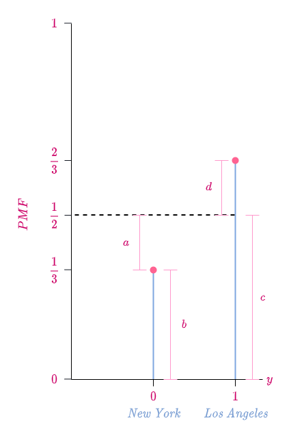
\end{equation*} The following diagram is a pictorial representation of the PMFs of X and Y. I have written the place that a particular random value corresponds to for the sake of clarity.

The following diagram illustrates the calculation of total variation distance.

We defined total variation distance as the maximum difference between the probabilities assigned to the same event by two distributions defined on the same sample space.
Looking at the PMFs of X and Y we find that they differ when their random values are either 0 \text{ or } 1 i.e., p_X(0) > p_Y(0) and p_Y(1) > p_X(1).
Let A be the event that either Ann or Kelly in is New York and B be the event that either Ann or Kelly is in Los Angeles. The event B is the same as event A^c since when Ann and Kelly are not in New York they are in Los Angeles.
Total variation distance is the maximum of \big|p_X(A) - p_Y(A)\big| and \big|p_X(A^c) - p_Y(A^c)\big|.
\big|p_X(A) - p_Y(A)\big| = \big|\frac{1}{2} - \frac{1}{3}\big| =\frac{1}{6}.
\big|p_X(A^c) - p_Y(A^c)\big| = \big|\frac{1}{2} - \frac{2}{3}\big| =\frac{1}{6}.
So the total variation distance = \frac{1}{6}.
This shows that in order to calculate the total variation distance we find an event in the sample space such that it maximizes the difference between the probabilities assigned to the same event by two distributions. How d0 we find this event?
We choose event A such that the probability of every outcome in event A in one distribution (here p_X) is greater than the probability of the corresponding outcome in event A in the other distribution (p_Y), i.e., p_X(A) > p_Y(A). Since p_X(0) > p_Y(0) (see diagram), so we choose A = \{0\}, namely, the event where either Ann or Kelly is in New York.
Consequently, in the other event A^c = \{1\}, the probability of every outcome in one distribution (p_X) is lesser than or equal to the probability of the corresponding outcome in the other distribution (p_Y), i.e., p_X(A^c) \leq p_Y(A^c).
Since in both the events A \text{ and } A^c, the probabilities of outcomes in one distribution is greater than or equal to the probabilities of outcomes in the other distribution (for A, p_X(A) > p_Y(A) and for A^c, p_Y(A^c) \geq p_X(A^c)), among all the possible subsets of the sample space, these are the only two events that could maximize the difference in probabilities that the two distributions assign to them.
Therefore the total variation distance is either \big|p_X(A) - p_Y(A)\big| \text{ or } \big|p_X(A^c) - p_Y(A^c)\big|. From the figure and our calculation it is seen that \big|p_X(A) - p_Y(A)\big| = \big|p_X(A^c) - p_Y(A^c)\big| = \frac{1}{6}. Is this always the case?
Yes, always \big|p_X(A) - p_Y(A)\big| = \big|p_X(A^c) - p_Y(A^c)\big|. Below we explain why.
By axiom of probability,
p_X(A) + p_X(A^c) = 1 and p_Y(A) + p_Y(A^c) = 1.
Hence, p_X(A) + p_X(A^c) = p_Y(A) + p_Y(A^c) \Rightarrow p_X(A) - p_Y(A) = p_Y(A^c) - p_X(A^c).
Since p_X(A) > p_Y(A) \text{ and } p_Y(A^c) \geq p_X(A^c),
\big|p_X(A) - p_Y(A)\big| = \big|p_X(A^c) - p_Y(A^c)\big|.
The following is a visual proof for why \big|p_X(A) - p_Y(A)\big| = \big|p_X(A^c) - p_Y(A^c)\big|.
By the axiom of probability,
p_X(A) + p_X(A^c) = 1 = p_Y(A) + p_Y(A^c).
Since A = \{0\} \text{ and } A^c = \{1\},
\begin{equation*}
\begin{split}
p_X(0) + p_X(1) & = p_Y(0) + p_Y(1) \\
\frac{1}{2} + \frac{1}{2} & = \frac{1}{3} + \frac{2}{3} \\
(a + b) + c & = b + (c + d) \\
\text{Cancelling } b + c \text{ from both sides,} \\
a & = d \\
\end{split}
\end{equation*}
Since in order to calculate total variation distance we have to find a particular subset (event), over all possible subsets of the sample space S, that maximizes the difference in probabilities between two distributions and though we found a good way to find this subset, is there a more straightforward way to calculate total variation distance?
Let us try and find an answer to this question.
We have already proved that,
\big|p_X(A) - p_Y(A)\big| = \big|p_X(A^c) - p_Y(A^c)\big|.
Since A = \{0\} \text{ and } A^c = \{1\},
\big|p_X(0) - p_Y(0)\big| = \big|p_X(1) - p_Y(1)\big| = \textit{Total Variation Distance}.
This implies,
\big|p_X(0) - p_Y(0)\big| + \big|p_X(1) - p_Y(1)\big| = 2 \times \textit{Total Variation Distance}.
We find that the left-hand side of the above equation is just a simple sum over the sample space S i.e., it is the sum of the absolute difference in probabilities that the two distributions assign to each outcome in the sample space. This measure is called the \mathcal{L_1} norm or \mathcal{L_1} distance.
\begin{equation*}
\begin{split}
\big\|p_X - p_Y\big\|_1 & = \sum_{i = 0}^{1} \big|p_X(i) - p_Y(i)\big| \\
& = \big|p_X(0) - p_Y(0)\big| + \big|p_X(1) - p_Y(1)\big| \\
& = 2 \times \textit{Total Variation Distance}
\end{split}
\end{equation*}
Therefore,
Total Variation Distance = \frac{\big\|p_X - p_Y\big\|_1}{2} = \frac{\mathcal{L_1} \text{ norm}}{2}.
Hence a simple way to calculate total variation distance would be to find the sum of the absolute difference in probabilities that the two distributions assign to each outcome in the sample space and then divide that sum by 2.
In our diagram,
Total Variation Distance = a = d ,
\mathcal{L_1} \text{ norm } = a + d .
Now that we have a sound intuition about total variation distance, in the next part we will give it a mathematically rigorous treatment.