Categories
mathematics Set Theory

Set Theory Primer

authored by Premmi and Beguène

We will briefly discuss some topics from set theory which we will encounter during our study of number theory and cryptography.

Mathematical Object

A mathematical object is an abstract entity, precisely defined, often in terms of other mathematical objects, and ultimately grounded in a set of axioms—fundamental assumptions that are taken as starting points within a particular mathematical theory.

Unlike physical objects that exist in the real world, mathematical objects exist only in the realm of ideas. This abstract nature is a key characteristic of mathematical objects. A physical chair is a concrete object, while the concept of a chair, which might be studied mathematically in terms of its shape or dimensions, is an abstract mathematical object.

These objects can represent a wide range of mathematical concepts, including:

  • Numbers: Integers (\text{e.g.,} -\!2, 0, 5), real numbers (\text{e.g., }\pi, \sqrt{2}), complex numbers (\text{e.g., }2 + 3i).

  • Sets: The empty set (\emptyset), the set of natural numbers (\mathbb{N} = \{1, 2, 3, \ldots\}).

  • Relations: “less than” (\text{e.g., }4 < 5).

  • Functions: e.g., f(x) = x^2.

  • Sequences: e.g., 1, 2, 4, 8, \ldots.

  • Geometric Objects: Points, lines, planes, triangles, spheres.

  • Abstract Structures: Groups, rings, fields.

Mathematical objects are characterized by their properties and by the relationships they have with other mathematical objects. They are the focus of mathematical study, and mathematicians explore and analyze them using the tools of mathematical logic.

While we often use informal language to talk about mathematical objects (e.g., “the number 2"), formal definitions are crucial for rigor. Within a specific mathematical theory, such as set theory, mathematical objects are defined precisely using the language of that theory. This distinction between formal and informal language is not merely a matter of style; it is essential for mathematical rigor and to avoid ambiguity.

Mathematical Theorems and Proofs

Mathematical objects are related to one another through the process of mathematical proof.

Axiom

The process of mathematical proof is central to mathematics. It’s how we establish mathematical truths with certainty. These proofs are ultimately based on a set of fundamental assumptions called axioms.

Axioms are fundamental assumptions that are taken as starting points within a particular mathematical theory. They are not proven within that theory itself, but rather serve as the foundation upon which all proofs within that theory are built. While historically some axioms were considered “self-evident”, modern mathematics emphasizes the role of axioms as postulates—accepted assumptions—rather than necessarily “obvious” truths. For example, the Peano Axioms, while fundamental, are not necessarily “self-evident” in the everyday sense. They are postulates that we accept as the basis for reasoning about natural numbers.

Different mathematical theories have different sets of axioms. For example, the Peano Axioms are a set of axioms that define natural numbers by including axioms that define zero, the successor function, and the principle of mathematical induction. Set theory, on the other hand, is a theory about sets and their properties. It is typically based on the Zermelo-Fraenkel axioms (ZF), which include axioms about the existence of the empty set, pairing, unions, power sets, and so on. These two theories, number theory and set theory, have entirely different sets of axioms because they are about fundamentally different kinds of mathematical objects.

Proof

A proof is a rigorous and logically sound argument that demonstrates the truth of a mathematical statement. These proofs are constructed step-by-step, with each step justified by an axiom, a previously proven theorem, or a rule of logic.

Theorem

A theorem is a mathematical statement that has been proven to be true. Theorems are important because they expand our knowledge of mathematical objects and their relationships. Once a statement has been proven to be a theorem, we can use it as a building block in the proofs of other theorems.

Lemma

A lemma is a preliminary theorem used in the proof of another, typically more significant, theorem.

Corollary

A corollary is a theorem that follows directly (and often easily) from another theorem.

Property

Mathematical objects have characteristics called properties that are fundamental to how we define, classify, reason about and prove theorems about them. A property is a characteristic that some mathematical objects possess. If an object possesses a particular property, then statements about that object based on that property are true.

Properties are often used to classify and distinguish mathematical objects. For instance, a circle is defined as the set of all points equidistant from a given point (its centre). Since this property is not shared by an ellipse, this difference allows us to classify them as distinct shapes.

Similarly, being divisible by 2 is a property of the number 6, classifying it as even and distinguishing it from odd numbers, which lack this property.

Here are further examples of properties for various mathematical objects:

  • Numbers: is prime, is positive, is greater than 5, is a perfect square, is rational

  • Sets: is finite, is a subset of, is empty, has cardinality n, is infinite

  • Functions: is continuous, is differentiable, is linear, is injective (one-to-one), is surjective (onto)

  • Geometric figures: is a triangle, is a circle, has an area greater than 12, is a square, is congruent to

For each property, the collection of all objects that satisfy the property is called its extension. For example, the extension of the property “is greater than 5" is the collection of all numbers which are greater than 5.

As we have discussed, mathematical objects are characterized by their properties. But the property “is even” is just a concept—an idea—that exists independently of how we represent it. It’s the idea of being divisible by 2. How do we determine with mathematical rigor whether an object has a particular property? We will do so using predicate—a formal statement that, when applied to an object, is true if and only if that object possesses the property it represents—which will be our next topic of discussion.

Predicate

When we talk about properties informally, we often use natural language. For example, we might say “The number 4 is even.” or “That shape is a triangle.” While these statements are understandable, they express specific instances of properties. Mathematical theorems and proofs are often about all objects of a certain type (e.g., all even numbers, all triangles, all continuous functions). We want to make statements that are universally true within a specific mathematical system. Therefore, for rigorous mathematical reasoning, we need to represent properties in a general and precise way. This is where predicates come in.

Definition

A predicate is a sentence containing one or more variables, each representing a mathematical object. This sentence becomes a proposition—a statement that is either true or false—only when specific values are assigned to those variables. Crucially, predicates serve as formal representations of properties, allowing us to determine whether a given object possesses that property. They act as formal tests or criteria for recognizing instances of the property.

While predicates with a single variable are used to represent properties of individual objects, predicates can also have multiple variables, allowing us to express relationships between objects. We will explore these relationships, called relations, in more detail later.

Truth Set and Universe of Discourse

The collection of objects that, when substituted for the variables in a predicate, makes it a true proposition is called the truth set of the predicate.

To determine the truth set, we must know which objects are available for consideration; that is, we must assume that a universe of discourse has been agreed upon (either explicitly or implicitly through context). Commonly used universes of discourse are the number systems which consist of the natural numbers (\mathbb{N}), integers (\mathbb{Z}), rational numbers (\mathbb{Q}), real numbers (\mathbb{R}), and complex numbers (\mathbb{C}).

With a universe specified, two predicates P(x) and Q(x) are equivalent if they have the same truth set.

For example, the predicates “5x + 7 = 17" and “x = 2" are equivalent predicates in any of the number systems we have mentioned above. On the other hand, “x^2 = 9" and “x = 3" are not equivalent when the universe is \mathbb{Z} because “x = -3" is also a solution to “x^2 = 9". However, they are equivalent when the universe is \mathbb{N} because we only consider positive integers..

Examples

Let’s illustrate how a predicate formalizes the property “evenness”.

Informally, we understand “evenness” as the characteristic of being divisible by 2. However, to work with this concept mathematically, we need a precise and general way to express it. We can use a predicate, often denoted as P(x), where x represents any mathematical object—in this case, an integer. Therefore, the universe of discourse is the collection of all the integers, usually represented as a set, which will be the topic of our next discussion. P(x) represents the sentence “x is divisible by 2”.

Now, P(x) is not a statement about a specific number. It’s a template or a rule that we can apply to any number. When we substitute a specific value for x, the predicate becomes a statement (or proposition) that is either true or false.  

For example, if we substitute x = 4, then P(4) becomes the proposition “4 is divisible by 2", which is true; if we substitute x = 5, then P(5) becomes the proposition “5 is divisible by 2", which is false. The truth set of P(x) is the set of all even integers.

The predicate P(x) itself is not true or false. It’s a formal representation of the property of evenness. It provides a precise way to test if a number has that property.

Similarly, the property of “being a triangle” can be represented by a predicate T(s), where s represents any geometric shape. T(s) represents the statement “s is a triangle”. If we substitute a triangle for s, T(s) becomes true. If we substitute a square, T(s) becomes false. Here the universe of discourse is set of all geometric shapes and the truth set of T(s) is the set of all triangles.

Functional Predicate

Among the various types of predicates, there is a special category known as functional predicates.  

A functional predicate is a predicate that represents a function. In essence, it’s a way to express a function’s behavior using the language of predicates. A functional predicate, often denoted as F(x, y), expresses the relationship between an input x and its corresponding output y of a function.  

The key characteristic of a functional predicate is that for every input x, there is a unique output y that makes the predicate true. This uniqueness is what distinguishes functional predicates from general predicates and allows them to accurately represent functions.

Universe of Discourse and Truth Set

For a functional predicate F(x, y), the Cartesian product X \times Y serves as the universe of discourse, where X is the domain and Y is the codomain of the corresponding function.

The truth set of F(x, y) is the collection of ordered pairs (x, y) chosen from the Cartesian product X \times Y that makes the predicate true. For example, for the functional predicate F(x, y): y = 2x with \mathbb{N} \times \mathbb{N} as the universe of discourse, the truth set includes pairs like (1, 2), (2, 4), (3, 6) and so on. We can see that for any given x value, there is only one possible y value that will make the predicate F(x, y) true.

Definition

A predicate F(x, y) with its universe of discourse as the Cartesian product X \times Y of sets X and Y is a functional predicate if and only if:

  • For every x \in X, there exists a y \in Y such that F(x, y) is true.

  • For every x \in X, if F(x, y) is true and F(x, z) is true, then y = z.

Examples

The following are some examples of functional predicates:

  • Linear Function: The function f(x) = 2x can be expressed as the functional predicate F(x, y): y = 2x.
    • If x = 3 and y = 6 then F(3, 6) is true.  
    • If x = 3 and y = 7 then F(3, 7) is false.

  • Quadratic Function: The function f(x) = x² + 1 can be expressed as the functional predicate F(x, y): y = x² + 1.
    • If x = 2 and y = 5 then F(2, 5) is true.
    • If x = 2 and y = 4 then F(2, 4) is false.

  • String Length Function: Let f(s) be a function that returns the length of a string s. This can be expressed as the functional predicate F(s, n): n \text{ is the length of string } s.
    • If s = \text{``hello"} and n = 5 then F(\text{``hello"}, 5) is true.
    • If s = \text{``hello"} and n = 4 then F(\text{``hello"}, 4) is false.

Connection to Functions

As we have seen in the previous examples, a function can always be expressed as a functional predicate, and conversely, a functional predicate defines a function. The truth set of a functional predicate F(x, y) is the function represented as a set of ordered pairs (x, y) that satisfy the predicate.

We have now explored the concept of functional predicates, which provide rigorous way to define functions using the language of predicates. Functional predicates play a crucial role in the foundations of mathematics, particularly in axiomatic set theory.

The concept of a set is one of the most fundamental concepts in mathematics, which are often defined using predicates. Therefore, we will now discuss sets and how they are defined.

Set

Sets are often considered fundamental building blocks from which many other mathematical objects can be constructed. In this section, we will provide a detailed exposition of what sets are.

set is defined as a collection of objects that is well-defined. By well-defined, we mean that it is possible to determine unambiguously whether an object is to be included in the set or not.

The concept of a set is very general. While, in principle, the objects in a set can be anything, in mathematics we are primarily interested in sets of mathematical objects. These can be numbers, geometric figures, functions, and so on.

There is no restriction on the number of objects in a set. It can be finite or infinite; it may contain just one object, or even none. Also, there is no requirement for uniformity in the type of object used to construct the set–a perfectly good set might consist of four numbers, two squares and a function.

To deal with all of the sets that arise in mathematics, it is easiest to develop first those general properties common to all sets, and then to apply them in more special situations.

Membership

The objects in the set are called elements or members of the set. The members themselves are said to belong to the set.

To express symbolically that an element x belongs to a set S, we write x \in S.

If x does not belong to S, we write x \notin S.

Equality of Sets

Though sets can be described in different ways, a set is ultimately determined by its members.

For example, if X is the set of solutions of the equation

x^2 -6x + 8 = 0

and Y is the set of even integers between 1 \text{ and } 5, then X \text{ and } Y both have precisely two members, 2 \text{ and } 4. This means that X \text{ and } Y are the same set.

Therefore, we say that two sets are equal if they have the same members.

Equality of two sets S \text{ and } T is expressed in the usual way by S = T, and if S \text{ and } T are not equal, we write S \neq T.

This apparently banal criterion for equality of sets has some interesting consequences, as we shall see shortly.

Defining Sets

Sets are usually denoted by capital letters in italic, such as X, Y, Z and lower-case letters such as x, y, z to represent numbers and other objects that are individual elements, rather than sets.

There are three ways of describing sets, namely, the Roster notation, semantic description and the set-builder notation.

Roster Notation

Roster or enumeration notation defines a set by listing its elements. The elements are listed between curly braces and separated by commas.

For example, S = \{1, 4, 7, 11\} means that S.is the set who members are the numbers 1, 4, 7, 11 and only these.

The basic relation in set theory is that of elementhood, or membership i.e., in a set all that matters is whether an element is in it or not; thus, the order or repetition of elements in the roster notation is irrelevant. For example, \{1, 2, 3\} \text{ and } \{3, 2, 3, 1\} represent the same set.

For sets with many elements, where the elements follow some implicit pattern, the list of elements can be abbreviated using an ellipsis, denoted by ‘…’. For example, the set of first hundred even numbers may be specified in roster notation as \{2, 4, 6, \ldots, 200\}.

To describe an infinite set in roster notation, an ellipsis is placed at the end of the list or at both ends to indicate that the list continues forever. For example, in roster notation, the set of positive integers is represented as \{1, 2, 3, \ldots\} and the set of integers is represented as \{\ldots,-3,-2,-1,0,1, 2, 3, \ldots\}.

When specifying a set, it may not be convenient, or even possible, to write down a complete list of all the members. For example, the set of prime numbers is better described precisely by that phrase, rather than by the list \{2, 3, 5, 7, 11, 13, 17, 19, \ldots\}. Indicating a few terms of an infinite set in this manner might be open to misinterpretation since the elements inside the braces need not be in any specific order. So this list may also be written as \{13, 17, 19, 2, 3, 7, 11, 5, \ldots\}. How could we be sure that this is the set of all primes?

As we saw with the set of prime numbers, roster notation can be inadequate for describing infinite sets or sets with complex membership criteria. Semantic description which we will discuss next provides a way to overcome this limitation.

Semantic Description

A semantic description of a set defines the set by using a sentence to specify the properties of objects contained in the set. This method of description does not list the elements of the set explicitly but rather provides a clear and unambiguous description of what the elements are or how they are determined.

For example, “Let X be the set of all the prime numbers.” is a valid semantic description. This clearly defines the set without listing all its elements.

We’ve seen how the semantic description describes a set as a collection of objects that share some common properties. As we have already discussed, these properties can be formalized using a mathematical predicate–-statement about an object that is either true or false depending on whether the object has the properties described by the predicate. Predicates provide the mathematical rigor needed to define the properties of objects concisely and precisely. Set-builder notation then uses these predicates to define sets in a very clear and compact way which will be our next topic of discussion.

Set-Builder Notation

A Formal Language for Defining Sets

While we can describe sets using roster notation (\text{e.g.,} \{1, 2, 3, 4\}) or semantic description (e.g., “the set of all prime numbers”), set-builder notation offers a precise and unambiguous way to define sets based on the properties their elements must satisfy.

Suppose we want to define the set of even numbers. We could start with the set of all integers and “filter” this set to keep only the even numbers. But how do we express this filtering process precisely and concisely? We do so using predicates—formal statements that are either true or false for a given object, depending on whether or not the object satisfies the property represented by the predicate. A predicate, therefore, acts as our “filter”, specifying the property an object must have to be included in our new set. Set-builder notation allows us to formally define sets based on these predicates, which, in turn, represent the properties of their elements.

A set S described in set-builder notation has the form

S = \big\{x \in X\,|\, P(x)\big\}

Let’s break down this notation:

  • \{\,\, \ldots \,\, \}: The curly braces denote a set. They enclose the description of the set’s elements.

  • x \in X: This part specifies that we are considering elements x that belong to a pre-existing set X. X is often called the parent set, universal set or universe of discourse. It defines the pool of potential elements from which we will select those that meet our criteria.

  • \big|: This vertical bar is read as “such that” or “for which.” It separates the generic element x from the condition P(x) it must satisfy. We can also use “:” instead of the vertical bar.

  • P(x): This is a predicate—a statement that can be either true or false for a given x. It expresses the property that elements of the new set must possess. It’s the “filter” that determines which elements from X are to be included in the set S.

In this notation, the description should be read as “S is the set of all x that are elements of X such that P(x) is true.”

Examples

Following are some examples of defining sets using set-builder notation:

  • Even Integers: Let \mathbb{Z} represent the set of all integers (our universe of discourse). We can define the set of even integers E as: E = \{x \in \mathbb{Z} \,|\, x \text{ is divisible by } 2\}. This reads as “E is the set of all x that are elements of \mathbb{Z} such that x is divisible by 2." The predicate P(x) here is “x is divisible by 2". It selects only those integers that are divisible by 2, effectively “filtering” the integers to get the even integers.

  • Squares of Natural Numbers: Let \mathbb{N} represent the set of natural numbers (our universe of discourse). The set of perfect squares S within the natural numbers can be defined as: S = \{x \in \mathbb{N} \,|\, \text{there exists a } y \in \mathbb{N} \text{ such that } x = y^2\}. This reads as “S is the set of all x that are elements of \mathbb{N} such that there exists a y that is also an element of \mathbb{N} for which x equals y squared.” This example demonstrates how set-builder notation can express more complex conditions using quantifiers (like “there exists”, denoted by \exists). The predicate here is “there exists a y \in \mathbb{N} \text{ such that } x = y^2".

    However, it’s important to note that this predicate, as written, is a tautology for any y. This means that for any x that is a perfect square, there will always be exactly one y in \mathbb{N} that satisfies x = y^2. While this representation is technically correct, it’s not the most efficient or intuitive. We will subsequently discuss better ways to represent this set using functions, which will lead to a more concise and clear notation.

  • Prime Numbers: Let \mathbb{N} be our universe of discourse again. The set of prime numbers P can be defined as: P = \{ p \in \mathbb{N} \,|\, p > 1 \text{ and for all } n \in \mathbb{N}, \text{if } n \text{ divides } p, \text{ then } n = 1 \text{ or } n = p\}. This example shows how to express a more complex mathematical property (primality) using set-builder notation.

  • A More Abstract Example: Let X be any set. We can define a set Y containing all elements that are not equal to a specific element z in X as: Y = \{x \in X \,|\, x \neq z\}. This reads as “Y is the set of all x that are elements of X such that x is not equal to z.”

  • Bounded Set of Reals: Let \mathbb{R} be the set of real numbers. We can define the set of real numbers between 0 \text{ and } 1 (inclusive) as: \{x \in \mathbb{R} \,|\, 0 \leq x \leq 1\}.
More Complex Expressions: Using Functions

In our previous examples of set-builder notation, we primarily saw cases where the elements of the set were directly taken from the parent set (also referred to as the universe of discourse). However, set-builder notation is much more flexible. We can also define sets where the elements are some transformations (represented as functions) of the elements from the parent set, and these resulting elements can be further filtered if required based on specific properties.We will explore functions in greater depth later, but for now, it’s important to understand that the left side of set-builder notation can represent a function of x denoted by f(x).

Consider the example of the set of perfect squares within the natural numbers:

S = \big\{x \in \mathbb{N} \,|\,  \text{there exists a } y \in \mathbb{N} \text{ such that } x = y^2\big\}

This notation expresses the set of perfect squares, but it can be rewritten using a function to make it more concise.

To express the set of perfect squares in set-builder notation using functions, we can define the function f(y) as f(y) = y^2 and the universe of discourse X as X = \mathbb{N}. Then, the set of perfect squares can be written in set-builder notation as:

S = \big\{y^2 \,|\, y \in \mathbb{N}\big\}

This reads as “the set of all y squared such that y is a natural number.”

This example demonstrates how the function form of set-builder notation can be used to define sets where the elements are functions of other elements.

A set S described in set-builder notation has the general form:

S = \big\{f(x) \,|\, x \in X \text{ and } P(x)\big\}

Here:

  • f(x) is a function that takes an element x as input and produces a value as output.
  • x \in X specifies that x belongs to a pre-existing set X (the universe of discourse).
  • P(x) is a predicate that specifies a condition that x must satisfy. This part is optional. If no additional condition is needed, it can be omitted.

Examples

Following are some examples of defining sets using the function form of set-builder notation:

  • Even Integers:
    • Let f(x) = 2x (the function) and X = \mathbb{Z} (the universe of discourse).
    • The set of even integers can be defined as \{2x \,|\, x \in \mathbb{Z}\}.
    • This reads as “the set of all 2x such that x is an integer.” Here, P(x) is omitted.

  • Odd Integers:
    • Let f(x) = 2x + 1 (the function) and X = \mathbb{Z} (the universe of discourse).
    • The set of odd integers can be defined as \{2x + 1 \,|\, x \in \mathbb{Z}\}.
    • This reads as “the set of all 2x plus one such that x is an integer.” Here, P(x) is omitted.

  • Squares of positive real numbers greater than 3:
    • Let f(x) = x^2, X = \mathbb{R} and P(x) be x > 3.
    • The set of squares of real numbers greater than 3 can be defined as \{x^2 \,|\, x \in \mathbb{R} \text{ and } x > 3\}.
    • This reads as “the set of all x squared such that x is a real number and x is greater than 3". Here P(x) \text{ is } x > 3.

  • Rational Numbers:
      • Let f(p, q) = p/q(the function of two variables), X = \mathbb{Z}, Y = \mathbb{Z} (universes of discourse) and P(q) be q \neq 0.
      • The set of rational numbers, \mathbb{Q}, can be defined as \{p/q \,|\, p,q \in \mathbb{Z} \text{ and } q \neq 0\}.
      • This reads as “the set of all p divided by q such that p is an integer and q is an integer not equal to 0". Here P(q) \text{ is } q \neq 0.

        When defining sets using functions in set-builder notation, the function doesn’t always have to have a single input. For example, to define the set of rational numbers \mathbb{Q}, we use the function f(p, q) = p/q, where p and q are integers. This function takes two inputs and produces a single output, which is the ratio of p and q. This is related to the concept of a binary operation, which we will discuss in more detail later.

    • Ordered Pairs Representing Odd Integers
      • Let f(t) = (t, 2t + 1) (the function creating ordered pairs) and X = \mathbb{Z} (the universe of discourse).
      • The set of ordered pairs representing odd integers can be defined as \big\{(t, 2t + 1) \,|\, t \in \mathbb{Z}\big\}.
      • This reads as “the set of all ordered pairs (t, 2t + 1) such that t is an integer.” Here, P(t) is omitted.

        This example demonstrates how set-builder notation can be used to create sets of ordered pairs, representing function mappings. Here, the function f(t) = (t, 2t + 1) takes an integer t and produces an ordered pair where the first element is t and the second element is 2t + 1, which is an odd integer. The ordered pair provides a specific association, pairing each integer t with its corresponding odd integer 2t + 1. For instance, when t = 0, the pair (0, 1) associates 0 with 1; when t = 1, the pair (1, 3) associates 1 with 3, and so on. This set visually represents the relationship between integers and odd integers as a set of pairs, which is a fundamental concept in defining functions as sets of ordered pairs.

    These examples illustrate the flexibility and power of set-builder notation. Set-builder notation allows us to define sets precisely and concisely either by selecting elements based on their specific properties from a pre-existing set (referred to as the universe of discourse) or by creating elements from a pre-existing set by transforming its elements using functions and optionally, further selecting from these transformed elements those that satisfy some specific properties. The universe of discourse could be a familiar number system or a more abstract set. The key is always to identify the parent set (also called the universe of discourse) and the criteria for membership in the new set, which may be specified by a predicate alone or by a function and an optional predicate.

    Proving Equality of Sets Defined by Set-Builder Notation

    As we have already discussed, two sets are equal if and only if they contain the same elements. When sets are defined using set-builder notation, their equality hinges on the equivalence of their defining rules, which encompass predicates, functions (if present) and domain specifiers (universes of discourse).

    We will now discuss how to determine the equality of these sets whose definition encompasses predicates, functions or both.

    Sets Defined by Predicates

    Specifically, given sets X \text{ and } Y, and predicates P(x) \text{ and } Q(x), we have:

    \big\{x ∈ X \,|\, P(x)\} = \{x ∈ Y \,|\, Q(x)\big\}
    \text{ if and only if}
    (\forall t)[(t \in X \land P(t)) \iff (t \in Y \land Q(t))]

    This means that the sets \{x \in X \,|\, P(x)\} and \{x \in Y \,|\, Q(x)\}, defined by the predicates P(x) and Q(x) on sets X and Y respectively, are equal if and only if for any element t, the combined conditions of t belonging to X and satisfying P(t) are logically equivalent to the combined conditions of t belonging to Y and satisfying Q(t).

    Therefore, to prove the equality of two sets defined by set-builder notation using predicates, it is sufficient to demonstrate the equivalence of their defining rules, including both the predicates and the domain qualifiers (universes of discourse).

    Example

    Consider the sets \{x \in \mathbb{R} \,|\, x^2 = 1\} and \{x \in \mathbb{Q} \,|\, |x| = 1\}.

    These sets are equal because the two rule predicates are logically equivalent as shown below.

    (x \in \mathbb{R} \wedge x^2 = 1) \iff (x \in \mathbb{Q} ∧ |x| = 1)

    This equivalence holds because, for any real number x, x^2 = 1 if and only if x is a rational number with |x| = 1. In particular, both sets are equal to the set \{-1, 1\}.

    Sets Defined by Functions

    Given two functions f(x) \text{ and } g(y) with sets X \text{ and } Y as their respective domains and predicates P(x) \text{ and } Q(y) with X \text{ and } Y as their respective universes of discourse, we have:

    \big\{f(x) \,|\, x \in X \wedge P(x) \big\} = \big\{g(y) \,|\, y \in Y \wedge Q(y) \big\}
    \text{if and only if}
    (\forall z \in Z) \big[(\exist x \in X) (f(x) = z \wedge P(x)) \iff (\exist y \in Y) (g(y) = z \wedge Q(y))\big]

    where Z is a set that contains all possible output values from f(x) \text{ and } g(y) i.e., Z is a set that includes the ranges of both functions.

    This means that for any element z \in Z, z is an element of \big\{f(x) \,|\, x \in X \wedge P(x) \big\} if and only if z is an element of \big\{g(y) \,|\, y \in Y \wedge Q(y) \big\}.

    Example

    Consider two sets A \text{ and} B defined as follows:

    • A = \{(2x + 1)^2 \,|\, x \in \{0, 1, 2\}\}

    • B = \{8y + 1 \,|\, y \in \{0, 1, 3\}\}

    Let us determine the elements of sets A \text{ and } B.

    • Set A
      • x = 0: (2(0) + 1)² = 1² = 1
      • x = 1: (2(1) + 1)² = 3² = 9
      • x = 2: (2(2) + 1)² = 5² = 25
      • Therefore, A = \{1, 9, 25\}
    • Set B
      • y = 0: 8(0) + 1 = 1
      • y = 1: 8(1) + 1 = 9
      • y = 3: 8(3) + 1 = 25
      • Therefore, B = \{1, 9, 25\}

    We can see that even though the functions used to define A \text{ and } B are different, and the domains are slightly different, the resulting sets are identical i.e., A = B.

    Conclusion

    Predicate Equivalence

    When sets are defined by predicates alone, their equality requires the logical equivalence of the predicates and domain specifiers.

    Function Equivalence

    When sets are defined by functions, their equality requires that for every possible output value z (within the combined range of the functions), z is in one set if and only if it is in the other. This ensures that the sets contain the same elements, even when the functions or universes of discourse are different.

    We’ve seen how set-builder notation allows us to define sets and prove their equality, using both predicates and functions. Now, it’s time to examine the axiomatic basis that makes this definition possible. The Axiom of Separation ensures the validity of set definitions using predicates, and the Axiom of Replacement does the same for sets defined through functions.

    The Theoretical Foundation: The Axiom of Separation

    Now that we have seen how set-builder notation works, it’s important to understand its theoretical basis. This notation is not just a convenient shorthand; it’s deeply rooted in the foundational principles of axiomatic set theory, specifically the Axiom of Separation. This axiom ensures that we can define new sets by selecting elements from existing sets using predicates, without running into logical contradictions like Russell’s Paradox.

    Russell’s Paradox highlights the dangers of unrestricted set formation. It considers the set R defined as “the set of all sets that do not contain themselves as elements.” This definition is based on the predicate “x is a set and x \notin x", which, when used to define R, leads to a contradiction as explained below.

    The Predicate: The core of Russell’s Paradox is the predicate P(x), which is defined as: P(x) = x \text{ is a set and } x \notin x. That is, P(x) is true if and only if x is a set and x is not an element of itself.

    Defining the Set R: Russell’s set R is then defined using set-builder notation based on this predicate: R = \{x \,|\, P(x)\} or equivalently, \{x \,|\, x \text{ is a set and } x \notin x\}. This reads as “R is the set of all x such that x is a set and x is not an element of itself.”

    The Paradox: The paradox arises when we ask: Is R an element of itself? In other words, is R \in R?

    • Case 1: Assume R \in R. If R is an element of itself, then by the definition of R \,(\text{and the predicate } P(x)\!), R must not be an element of itself. This is a contradiction.

    • Case 2: Assume R \notin R. If R is not an element of itself, then R satisfies the predicate P(x) (because R is a set and R \notin R). Therefore, by the definition of R, R must be an element of itself. This is also a contradiction.

    The Problem: Since both R \in R and R \notin R lead to contradictions, the very definition of R is problematic and the assumption that R is a set is not valid. It shows that we cannot define sets completely arbitrarily. The unrestricted use of predicates to define sets can lead to inconsistencies.

    Why the Axiom of Separation Helps:

    The Axiom of Separation avoids this paradox by restricting set formation. Instead of allowing us to define sets using any predicate, it requires us to start with an existing set X and then use a predicate to select elements from this set X to form a new set . This prevents us from creating sets like R that attempt to include “all sets” without a clearly defined parent set or universe of discourse, which is what leads to the self-referential paradox. The “x \in X" part of the set-builder notation in conjunction with the Axiom of Separation is what prevents the problematic self-reference. We are always building sets from existing sets, never creating sets “from thin air” that could lead to these kinds of contradictions. This is the key idea behind the Axiom of Separation, which states:

    For any set X and any predicate P(x), there exists a set Y such that for all x, x \in Y if and only if (x ∈ X \text{ and } P(x)).

    In simpler terms: Given a set X (often called the “parent set” or “universe of discourse”) and a predicate P(x) which expresses a property, we can form a new set Y containing precisely those elements of X that satisfy P(x). This axiom is crucial because it emphasizes that we always form new sets by selecting elements from existing sets. We don’t create sets from nothing, which is essential for avoiding paradoxes like Russell’s Paradox.

    Additionally, this axiom highlights the connection between sets and predicates. For instance, given any set that is defined by selecting elements from an existing set, we can define a predicate that determines membership in this set. This demonstrates that any set defined from an existing set can be represented by a predicate. Thinking about this equivalence naturally leads to a more abstract question about the nature of mathematical objects themselves. Are sets primary, and properties merely ways to delineate them, or do the underlying properties hold a more fundamental status? This is a rich area of philosophical debate within mathematics, though we will not delve into it further here.

    This grounding in the Axiom of Separation provides a solid foundation for set-builder notation, ensuring its consistency and reliability as a tool for defining sets in mathematics. It should be noted that the Axiom of Separation is a cornerstone of Zermelo-Fraenkel set theory (ZFC), the most commonly used foundation for mathematics. It’s worth noting that other axiomatic set theories exist, some of which handle the concept of sets and potential paradoxes in different ways.

    Axiom of Replacement

    It is important to note that the Axiom of Separation, as stated, primarily addresses the creation of new sets from existing sets based on predicates. However, when using functions within set-builder notation, an additional foundational principle comes into play: the Axiom of Replacement.

    The Axiom of Replacement asserts that if F(x, y) is a functional predicate (meaning that for every x, there is a unique y such that F(x, y) is true), and X is a set, then there exists a set Y such that for every x \in X, there is a y \in Y such that F(x, y) is true. In simpler terms, this axiom allows us to create a new set by applying a function to each element of an existing set.

    Therefore, when using functions in set-builder notation, we are implicitly utilizing both the Axiom of Replacement and the Axiom of Separation. First, the Axiom of Replacement guarantees the existence of a set containing the transformed elements resulting from applying a function f(x) to the elements of the initial set X. Subsequently, the Axiom of Separation allows us to filter (if required) these transformed elements based on a predicate P(f(x)), creating the final set as defined by the set-builder notation.

    In essence, the Axiom of Replacement handles the function application aspect, while the Axiom of Separation handles the filtering based on predicates. This dual application of axioms provides the complete theoretical foundation for defining sets using functions and predicates within set-builder notation.

    Our discussion of set-builder notation and its axiomatic foundations, focused on creating sets from existing sets. We will now discuss in detail these sets which are referred to as subsets.

    Subsets

    A set X is a subset of a set Y, written X \subset Y, if and only if every element of X is an element of Y.

    If X is a subset of a set Y, we can also express this relationship as Y \supset X, indicating that Y is a superset of X.

    For example, the set of positive integers \mathbb{Z}^+, is a subset of the set of integers \mathbb{Z} i.e., \mathbb{Z}^+ \subset \mathbb{Z}. Since every positive integer is also an integer, it follows that every element of \mathbb{Z}^+ is also an element of \mathbb{Z}. Thus, we can also write \mathbb{Z} \supset \mathbb{Z}^+ and refer to \mathbb{Z} as a superset of \mathbb{Z}^+.

    Proving Equality of Sets

    Sets are defined by their elements, so intuitively, two sets are equal if they contain exactly the same elements. However, while doing mathematical proofs, this insight does not directly provide a methodology for showing that two sets are equal. Therefore, to prove the equality of two sets, we take recourse to the concept of subsets.

    Any two sets X \text{ and } Y are equal if they contain exactly the same elements. If sets X \text{ and } Y contain the same elements, then every element of set X is an element of set Y and every element of Y is also an element of X i.e., X \subset Y and Y \subset X. Therefore, if X \text{ and } Y are to be equal as sets, then X \subset Y and Y \subset X. Thus, in a proof, to show that X = Y, we must show that X \subset Y and Y \subset X.

    The Empty Set

    The most basic set is the collection of no objects. This set is called the empty set or null set and is denoted by \varnothing \text{ or } \{\} to indicate that it contains no elements.

    From the definition of subset, it follows that the empty set \varnothing is a subset of set S if x \in \varnothing implies x \in S. Since the empty set contains no elements, the conditional statement “if x \in \varnothing implies x \in S” is vacuously true. Therefore, the empty set \varnothing is a subset of every set S i.e., \varnothing \subset S, for every set S.

    Unordered Pair

    Marie has two pens, one in red and another in yellow. If she is asked to list the colors of the pens she has, she can either list them as \{\text{red, yellow}\} or \{\text{yellow, red}\}. The order she lists them doesn’t matter since both the lists convey the same information. Such a pair where the order in which the elements are listed is irrelevant is called an unordered pair.

    Definition

    An unordered pair is a set of the form \{x, y\}, i.e., a set having two elements x \text{ and } y such that,
    \{x, y\} = \{y, x\} \text{ and } x \neq y.

    An unordered pair is a finite set of cardinality 2.

    Unordered n-tuple

    Suppose instead of 2 pens, Marie has 10 pens each of a different color. How would she list the colors of the 10 pens? The mathematical structure she would now use is called an unordered n-tuple.

    More generally, the concept of unordered pair can be extended to a set consisting of more than 2 elements i.e., one consisting of n elements, where n is some positive integer.

    An unordered n-tuple is a set of the form \{x_1, x_2, \ldots, x_n\} i.e., a set consisting of n distinct elements where the order in which the elements appear in the set is insignificant.

    Ordered Pair

    Marie takes two exams, one in English and another in Mathematics. When she is asked to list her scores in English and Mathematics, the order in which she lists them matters unless she got the same score in both the exams. The mathematical structure which Marie will now use is called an ordered pair.

    Definition

    An ordered pair (x, y) is a pair of mathematical objects where the order in which the objects appear in the pair is significant.

    That is, in general (x, y) \neq (y, x); (x, y) = (y, x) if and only if x = y.

    In the ordered pair (x, y), the object x is called the first entry and the object y, the second entry of the pair. Alternatively, the objects are also referred to as first and second components, first and second coordinates or the left and right projections of the ordered pair.

    Cartesian products and binary relations are defined in terms of ordered pairs.

    The Cartesian product of two sets X \text{ and } Y is the set of all ordered pairs whose first entry is in set X and whose second entry is in set Y\!\!, and is written as X \times Y.

    A binary relation, R, between sets X \text{ and } Y is a subset of X \times Y, i.e., R \subseteq X \times Y.

    Defining property of an ordered pair

    For any two ordered pairs, (x, y) \text{ and } (u, v), the characteristic (or defining) property of the ordered pair is

    (x, y) = (u, v) \text{ if and only if } x = u \text{ and } y = v

    That is, the ordered pair (x, y) should be defined in such a way that the above relation holds good. Any definition that has this property will do.

    We will next construct a definition of an ordered pair such that it satisfies this property.

    Defining the ordered pair using set theory

    Since we believe that set theory is the foundation of mathematics, where possible, we will always define mathematical objects as sets. Hence, we will define an ordered pair as a set. We will construct a set-theoretic definition of the ordered pair and prove that this definition satisfies the characteristic property of the ordered pair.

    Set-theoretic definition of an ordered pair

    The standard set-theoretic definition of the ordered pair (x, y) is, (x, y) := \{\{x\}, \{x, y\}\}.

    It should be noted that this definition is valid even when the first and second entries of the ordered pair are identical. That is,

    (x, x) = \{\{x\}, \{x, x\}\} = \{\{x\}, \{x\}\} = \{\{x\}\}.

    The definition of ordered pair satisfies the characteristic property of the ordered pair

    We have to prove that the definition of ordered pair satisfies the characteristic property of the ordered pair, namely,

    (x, y) = (u, v) \text{ if and only if } x = u \text{ and } y = v

    where (x, y) \text{ and } (u, v) are ordered pairs.

    Proof:

    First, we will assume that x = u \text{ and } y = v and prove that (x, y) = (u, v) under this assumption.

    By definition,

    (x, y) = \{\{x\}, \{x, y\}\}.

    Since x = u \text{ and } y = v,

    (x, y) = \{\{x\}, \{x, y\}\} = \{\{u\}, \{u, v\}\} = (u, v). (by definition of ordered pair)

    Next, we will prove that x = u \text{ and } y = v under the assumption (x, y) = (u, v).

    Either x = y \text{ or } x \neq y. We will do the proof for each of these cases.

    When x = y :

    (x, y) = \{\{x\}, \{x, y\}\} = \{\{x\}, \{x, x\}\} = \{\{x\}, \{x\}\} = \{\{x\}\}.

    \{\{u\}, \{u, v\}\} = (u, v) = (x, y) = \{\{x\}\}.

    This implies that \{u\} = \{u, v\} = \{x\} so that \{\{u\}, \{u, v\}\} = \{\{x\}, \{x\}\} = \{\{x\}\}.

    Since \{u\} = \{x\}, it implies that x = u.

    Also, since \{u, v\} = \{x\} and x = u, it must be the case that x = v so that \{u, v\} = \{x, x\} = \{x\}.

    We have so far proved that x = u \text{ and } x = v.

    By our hypothesis, x = y. Therefore, y = v.

    Thus we have proved that, for the case x = y, if (x, y) = (u, v) then x = u \text{ and } y = v.

    When x \neq y :

    (x, y) = (u, v) implies \{\{x\}, \{x, y\}\} = \{\{u\}, \{u, v\}\} (by definition of ordered pair).

    Suppose \{u, v\} = \{x\}. This implies that u = v = x so that \{u, v\} = \{x, x\} = \{x\}.

    Consequently, \{\{u\}, \{u, v\}\} = \{\{x\}, \{x, x\}\} = \{\{x\}, \{x\}\} = \{\{x\}\}.

    Since \{\{x\}, \{x, y\}\} = \{\{u\}, \{u, v\}\} and \{\{u\}, \{u, v\}\} = \{\{x\}\}, \{\{x\}, \{x, y\}\} = \{\{x\}\}.

    If \{\{x\}, \{x, y\}\} = \{\{x\}\} then x = y so that \{\{x\}, \{x, y\}\} = \{\{x\}, \{x, x\}\} = \{\{x\}, \{x\}\} = \{\{x\}\}.

    But this contradicts our assumption that x \neq y.

    Consequently, \{u, v\} \neq \{x\}.

    Suppose \{u\} = \{x, y\}. Then u = x = y so that \{u\} = \{x, y\} becomes \{x\} = \{x, x\} = \{x\}.

    But this result contradicts our assumption that x \neq y.

    Hence \{u\} \neq \{x, y\}.

    Therefore, \{x\} = \{u\}, which implies that x = u and \{x, y\} = \{u, v\}.

    If y = u then x = y which contradicts our hypothesis that x \neq y. Hence, y = v.

    We have thus proved that if (x, y) = (u, v) then x = u \text{ and } y = v.

    We have shown that our definition of ordered pair holds good.

    That is, (x, y) := \{\{x\}, \{x, y\}\} satisfies the defining property of an ordered pair, namely,

    (x, y) = (u, v) \leftrightarrow (x = u) \wedge (y = v).

    This definition of ordered pair adequately embodies the notion of order because (x, y) = (y, x) is false unless x = y.

    Tuple

    A tuple is a finite enumerated collection of mathematical objects in which repetitions are allowed and order matters. The mathematical objects in a tuple are referred to as the elements of the tuple.

    An n-tuple is a tuple of n elements, where n is a non-negative integer.

    There is only one 0\text{-tuple}, called the empty tuple. A 1\text{-tuple} is called a singleton, a 2\text{-tuple}, an ordered pair and a 3\text{-tuple}, a triple.

    Tuples are usually written by listing the elements within parenthesis and the elements are separated from one another by a comma and a space; for example, (7, 8, 9) denotes a 3\text{-tuple} otherwise called a triple. Sometimes instead of parenthesis, a square or angle brackets are also used to enclose the elements of a tuple. For example, \big[7, 8, 9\big] and \big<7, 8, 9\big> are valid representations of tuples.

    Defining properties of an n-tuple

    Two n\text{-}tuples (x_1, x_2, \ldots, x_n) and (y_1, y_2, \ldots, y_n) are equal if and only if x_1 = y_1, x_2 = y_2, \ldots, x_n = y_n.

    Consequently, a tuple differs from a set in the following ways :

    • A tuple may contain multiple instances of the same element, so tuple (4, 5, 6, 6, 7) \neq (4, 5, 6, 7); but set \{4, 5, 6, 6, 7\} = \{4, 5, 6, 7\}.

    • Tuple elements are ordered. Tuple (4, 5, 6) \neq (6, 5, 4) but set \{4, 5, 6\} = \{6, 5, 4\}.

    • A tuple has a finite number of elements while a set may have an infinite number of elements, for example, the set of integers.
    Definition of n-tuple

    There are several definitions of tuples that satisfy the properties enumerated above. However, since we have already defined the notion of an ordered pair, we will define an n\text{-}tuple recursively by starting from an ordered pair. An n\text{-}tuple can be viewed as an ordered pair with its first element corresponding to the first element of the ordered pair and its remaining n - 1 elements corresponding to the second element of the ordered pair. This definition can then be recursively applied to the (n - 1)\text{-}tuple.

    N-tuple defined as a nested ordered pair

    The following is a way to model tuples in Set Theory as nested ordered pairs :

    1. The 0\text{-}tuple (i.e., the empty tuple) is represented by the empty set \emptyset.

    2. An n\text{-}tuple with n > 0 can be defined as an ordered pair of its first entry and an (n-1)\text{-}tuple which contains the empty set, \emptyset, when n = 1 and the remaining entries when n > 1. That is,

      (x_1, x_2, x_3, \ldots, x_n) = (x_1, (x_2, x_3, \ldots, x_n))

    This definition can be applied recursively to the (n-1)\text{-}tuple as follows :

    (x_1, x_2, x_3, \ldots, x_n) = (x_1, (x_2, (x_3, (\ldots, (x_n, \emptyset) \dots)))).

    For example,

    (4, 5, 6) = (4, (5,6)) = (4, (5, (6, \emptyset)))
    

    An alternate way to define an n\text{-}tuple as a nested ordered pair is as follows :

    1. The 0\text{-}tuple (i.e., the empty tuple) is represented by the empty set \emptyset.

    2. For n > 0 :

      (x_1, x_2, x_3, \ldots, x_n) = ((x_1, x_2, x_3, \ldots, x_{n-1}), x_n).

    This definition can be applied recursively as follows :

    (x_1, x_2, x_3, \ldots, x_n) = ((\ldots(((\emptyset, x_1), x_2), x_3), \dots), x_n).

    For example,

    (4, 5, 6) = ((4, 5),6) = (((\emptyset, 4), 5),6)

    Cartesian Product

    Marie is hungry after a rigorous session of mathematics 😜 and decides to have lunch. She wants to have a main course followed by a dessert. She has 3 options for main course and 3 options for dessert as shown below.

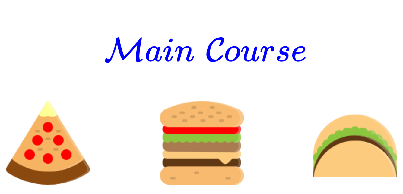
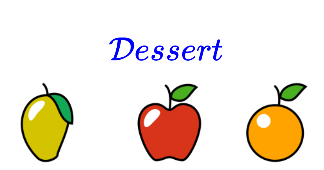
    We can view Marie having lunch as a procedure comprising of 2 steps with 3 options for step 1 and after the completion of step 1 there are 3 options for step 2 as shown below.

    What are the various possible ways that Marie can have lunch by choosing 1 main course and 1 dessert? We can answer this question by constructing a set of all ordered pairs (x, y) where x is one of the three possible choices for the main course and similarly, y for the dessert. Such a set of all possible ordered pairs where each ordered pair comprises of the first element from the first set and the second element from the second set is called the Cartesian product of two sets.

    Also, since there are 3 options for main course and 3 for dessert, the number of ways Marie could have her lunch is 3 \times 3 = 9 ways. So the set of all possible ordered pairs consists of 9 ordered pairs.

    This is illustrated below.

    Definition

    The Cartesian product of two sets X \text{ and } Y, denoted by X \times Y, is the set of all ordered pairs (x, y), where x belongs to X and y belongs to Y.

    That is,

    X \times Y = \{(x, y) : x \in X \text{ and } y \in Y\}

    Properties of Cartesian Product

    Non-commutativity

    For any two sets X \text{ and } Y, the Cartesian product X \times Y is not commutative. That is,

    X \times Y \neq Y \times X

    because the order of elements in the ordered pair is reversed unless at least one of the following conditions is satisfied, namely, X = Y or X \text{ or } Y is an empty set.

    Let us consider the following examples to illustrate the non-commutativity of X \times Y.

    Suppose X = \{4, 5\} \text{ and } Y = \{6, 7\}. Then,

    \begin{equation*} 
    \begin{split}
    X \times Y &= \{4, 5\} \times \{6, 7\} = \{(4, 6), (4, 7), (5, 6), (5, 7)\} \\
    Y \times X &= \{6, 7\} \times \{4, 5\}= \{(6, 4), (6, 5), (7, 4), (7, 5)\} \\
    \end{split}
    \end{equation*} 

    We can see that X \times Y \neq Y \times X because for all (x, y) \in X \times Y, x \neq y \text{ and consequently, }(x, y) \neq (y, x) .

    Now, suppose X = Y = \{4, 5\}. Then,

    \begin{equation*} 
    \begin{split}
    X \times Y &= \{4, 5\} \times \{4, 5\} = \{(4, 4), (4, 5), (5, 4), (5, 5)\} \\
    Y \times X &= \{4, 5\} \times \{4, 5\} = \{(4, 4), (4, 5), (5, 4), (5, 5)\} \\
    \end{split}
    \end{equation*} 

    In this case, X \times Y = Y \times X because X = Y.

    Finally, suppose X = \{4, 5\} \text{ and } Y = \emptyset. Then,

    \begin{equation*} 
    \begin{split}
    X \times Y &= \{4, 5\} \times \emptyset = \emptyset \\
    Y \times X &= \emptyset \times \{4, 5\} = \emptyset \\
    \end{split}
    \end{equation*} 

    In this case, X \times Y = Y \times X = \emptyset.

    Non-associativity

    The Cartesian product is not associative unless one of the involved sets is empty. That is,

    (X \times Y) \times Z \neq X \times (Y \times Z)

    where X, Y \text{ and } Z are sets.

    For example, suppose X = \{1\}, Y = \{2\} \text{ and } Z = \{3\}. Then,

    \begin{equation*} 
    \begin{split}
    (X \times Y) \times Z &= \big(\{1\} \times \{2\}\big) \times \{3\}  = \Big(\big\{(1, 2)\big\}\Big) \times \{3\} = \Big\{\big((1, 2), 3\big)\Big\}\\
    X \times (Y \times Z) &= \{1\} \times \big(\{2\} \times \{3\}\big) = \{1\} \times \Big(\big\{(2, 3)\big\}\Big) = \Big\{\big(1, (2,3)\big) \Big\} \\
    \end{split}
    \end{equation*} 

    We can see that (X \times Y) \times Z \neq X \times (Y \times Z).

    Cartesian Products of Several Sets

    n-ary Cartesian Product

    Marie is really really hungry 😧 and would like to have more than 2 courses for lunch. Now her lunch consists of n courses, where n is a positive integer greater than 2, with m_1 options for the first course (course 1) and after the completion of course i-1 \, (\text{where } i = 2, \ldots, n), there are m_i options for course i and so on till the n courses are completed. In this case, all the possible ways she could have her lunch could be represented as a set of ordered n\text{-}tuples called the n\text{-}ary Cartesian product defined over n sets, where each set enumerates the various options available for a particular course and each n\text{-}tuple represents one specific way in which Marie could lunch.

    In general, whenever a task can be decomposed into n steps, where n is a positive integer greater than 1, with m_1 options for step 1 and after completion of step i-1 \, (\text{where } i = 2, \ldots, n), there are m_i options for step i and so on till the n steps are completed, then all the possible ways the task could be completed can be enumerated as a set of ordered n\text{-}tuples called the n\text{-}ary Cartesian product defined over n sets, where each set enumerates the various options available to complete a particular step and each n\text{-}tuple is an enumeration of one particular way to perform the task.

    Definition

    The n\text{-}ary Cartesian product over n non-empty sets X_1, \ldots, X_n is defined as the set

    X_1 \times \ldots \times X_n = \big\{(x_1, \ldots, x_n) \,\,|\,\, x_i \in X_i \text{ for every } i \in \{1, \dots, n\}\big\}

    of n\text{-}tuples.

    n-ary Cartesian Power

    The Cartesian square of a set X is the Cartesian product X^2 = X \times X.

    For example, the 2\text{-}dimensional space (also called a plane) \mathbb{R}^2 = \mathbb{R} \times \mathbb{R} where \mathbb{R} is the set of real numbers is a Cartesian square on the set \mathbb{R}; \mathbb{R}^2 is the set of all points (x, y) on the plane, where x and y are real numbers.

    The n\text{-}ary Cartesian power of set X, denoted by X_n, is defined as

    X^n = \underbrace{X \times X \times \ldots \times X}_{n} = \big\{(x_1, \ldots, x_n) \,\,|\,\, x_i \in X \text{ for every } i \in \{1, \dots, n\}\big\}

    For example, the 3\text{-}ary Cartesian power of set \mathbb{R} where \mathbb{R} is the set of real numbers, is the 3\text{-}dimensional space
    \mathbb{R}^3 = \mathbb{R} \times \mathbb{R} \times \mathbb{R}; \mathbb{R}^3 is the set of all points (x, y, z) on the 3\text{-}dimensional space, where x, y and z are real numbers.

    More generally, \mathbb{R}^n, the n\text{-}ary Cartesian power of set \mathbb{R} where \mathbb{R} is the set of real numbers is the set of all points (x_1, \ldots, x_n) on the n\text{-}dimensional space, where x_i \in \mathbb{R \text{ for every } i \in \{1, \dots, n\}}.

    Cardinality of Cartesian Product

    Suppose Marie has 3 courses for lunch; there are 4 options to choose from for the first course, 3 options for the second course and 5 options for the third course. We have already seen that all the possible ways she could have her lunch is the Cartesian product defined over the 3 sets, each set representing a course. The number of possible ways she could have her lunch is the number of elements in this Cartesian product over the 3 sets which is equal to the product of the number of elements in each of the 3 sets i.e., 4 \times 3 \times 5 = 60.

    More generally, if a procedure can be broken into n steps such that here m_1 options for step 1 and upon completion of step i-1 where i = 2, \ldots, n, there are m_i options for step i and so on till the n\text{th} step is completed, then the number of ways of performing the procedure is m_1 \times m_2 \times \ldots \times m_n.

    In set-theoretic terms, if sets X_1, X_2, \ldots, X_n are finite, then

    |X_1 \times X_2 \times \ldots \times X_n| = |X_1| \cdot|X_2| \cdot \ldots \cdot |X_n|

    where |X_1 \times X_2 \times \ldots \times X_n| denotes the cardinality of the n\text{-}ary Cartesian product defined over n sets; the cardinality of a set is equal to the number of elements in the set.

    That is, the cardinality of the n\text{-}ary Cartesian product defined over n sets is equal to the product of the cardinalities of the n sets over which it is defined.

    Binary Relation

    Suppose we have a set of four actors, A = \{\text{Tom Cruise, George Clooney, Timothée Chalamet, Anne Hathaway}\} and a set of three movies, M = \{\text{Mission Impossible, Midnight in Paris, Dune}\}.

    A possible relation on A \text{ and } M is the relation “acted in”, given by

    R = \{(\text{Tom Cruise, Mission Impossible}), (\text{Timothée Chalamet, Dune}) \}

    That is, Tom Cruise acted in Mission Impossible and Timothée Chalamet acted in Dune. George Clooney and Anne Hathaway did not act in any of the movies in the set M and the movie Midnight in Paris did not feature any of the actors in set A.

    We can see that the set R associates elements of set A with the elements of set M.

    The set R could therefore be viewed as a subset of the Cartesian product of the two sets A \text{ and }M denoted by A \times M, which is the set of all ordered pairs (a, m) where a belongs to set A and m belongs to set M. That is,

    A \times M = \{(a, m) \,|\, a \in A \text{ and } b \in B\}

    Therefore,

    \begin{equation*} 
    \begin{split}
    A \times M &= \{(\text{Tom Cruise, Mission Impossible}), (\text{Tom Cruise, Midnight In Paris}), (\text{Tom Cruise, Dune}), \\
    &\quad\quad(\text{George Clooney, Mission Impossible}), (\text{George Clooney, Midnight In Paris}), (\text{George Clooney, Dune}), \\
    &\quad\quad(\text{Timothée Chalamet, Mission Impossible}), (\text{Timothée Chalamet, Midnight In Paris}), (\text{Timothée Chalamet, Dune}), \\
    &\quad\quad(\text{Anne Hathaway, Mission Impossible}), (\text{Anne Hathaway, Midnight In Paris}), (\text{Anne Hathaway, Dune}) \}
    \end{split}
    \end{equation*} 

    We can see that R \subseteq A \times M.

    A binary relation associates elements of one set, called the domain, with elements of another set, called the codomain.

    A binary relation over sets X \text{and } Y is a new set of ordered pairs (x, y) consisting of elements x from X and y from Y. That is, an element x is related to an element y if and only if the pair (x, y) belongs to the set of ordered pairs that defines the binary relation.

    It should be noted that the binary relation R over sets X and Y can be defined solely as a set of ordered pairs (x, y) where x \in X and y \in Y, without specifying the underlying relationship between x and y. That is, a binary relation R over sets X \text{ and } Y does not require a specific reason to relate or associate x \in X to y \in Y.

    In the example above, the following is another binary relation R over sets A \text{ and } M.

    R = \{(\text{George Clooney, Midnight In Paris}), (\text{Anne Hathaway, Dune}), (\text{Tom Cruise, Mission Impossible})\}

    R \subseteq A \times M but does not specify the relationship between the actor and the movie in each of its ordered pair i.e., the binary relation R over sets A \text{ and } M does not specify why a \in A relates to m \in M.

    Definition

    A binary relation R over sets X \text{and } Y is a subset of the Cartesian product X \times Y i.e., R \subseteq X \times Y.

    The set X is called the domain of R and the set Y is called the codomain of R.

    The statement (x, y) \in R reads “x is R-related to y” and is denoted by xRy.

    When X = Y, a binary relation is called a homogeneous relation or endorelation.

    In a binary relation, the order of elements is important i.e., if x \neq y then yRx can be true or false independently of xRy. For example, 2 divides 8 but 8 does not divide 2.

    Types of Binary Relations

    The following are some important types of binary relations over sets X \text{ and } Y.

    Function

    A function, denoted by f, is a special type of binary relation over sets X \text{ and } Y that satisfies the following conditions:

    • For every x \in X there exists y \in Y such that (x, y) \in f

    • (x, y) \in f \text{ and } (x, z) \in f imply that y = z

    A function is also called a map or mapping.

    Since f is a binary relation over sets X \text{ and } Y \!\!\text{,} it follows that it is a subset of their Cartesian product, X \times Y i.e., f \subseteq X \times Y. This relationship is usually written as f : X \rightarrow Y and read as “f is a function from X \text{ to } Y \text{"} or “f maps X \text{ to } Y \text{"}. The set X is called the domain of f and the set Y is called the codomain of f.

    When (x, y) \in f, we write y = f(x). We say that y is the image of f at x (or value of f \text{ at } x) and that x is a pre-image of y.

    Homogeneous Relation

    A homogeneous relation over a set X is a binary relation over X and itself i.e., it is a subset of the Cartesian product X \times X. This is commonly phrased as “a relation on X” or “a binary relation over X\text{"}.

    Some important properties that a homogeneous relation R over a set X may have are :

    Reflexive

    A binary relation R on a set X is reflexive if it relates every element of X to itself i.e., for all x \in X, xRx, where the notation xRx means that (x, x) \in R.

    For example, “is equal to” is a reflexive relation on the set of real numbers since every real number is equal to itself.

    Irreflexive

    A binary relation R on a set X is irreflexive if it does not relate any element of X to itself i.e., if xRx holds for no x \in X. This means that for all x \in X, (x, x) \not \in R.

    For example, “is greater than” is an irreflexive relation on the set of real numbers since there is no real number which is greater than itself.

    A relation is irreflexive if and only if its complement in X \times X is reflexive.

    For example, “is less than or equal to” is a reflexive relation on the set of real numbers, while its complement “is greater than” is an irreflexive relation.

    It should also be noted that not every relation which is not reflexive is irreflexive i.e., it is possible to define relations where some elements are related to themselves but others are not.

    For example, the binary relation “the product of x \text{ and }y is even” is reflexive on the set of even numbers, irreflexive on the set of odd numbers and neither reflexive nor irreflexive on the set of integers.

    Symmetric

    A binary relation R on a set X is symmetric if for all x, y \in X, \text{ if } xRy \text{ then } yRx.

    That is, if (x, y) \in R \text{ then } (y, x) \in R \text{ for all } x, y \in X.

    For example, “is parallel to” is a symmetric relation on the set of all lines in the Euclidean plane because for any two lines \overleftrightarrow{AB} \text{ and } \overleftrightarrow{CD}, if \overleftrightarrow{AB} \parallel \overleftrightarrow{CD} is true, then \overleftrightarrow{CD} \parallel \overleftrightarrow{AB} is also true.

    Antisymmetric

    A binary relation R on a set X is antisymmetric if there is no pair of distinct elements of X each of which is related by R to the other.

    That is, R is antisymmetric if for all x, y \in X,

    if xRy with x \neq y then yRx must not hold,

    or equivalently,

    if xRy \text{ and } yRx \text{ then } x = y.

    The divisibility relation on the set of positive integers is antisymmetric. If m \text{ and } n are two positive integers which are distinct, then if m divides n, then n cannot divide m. For example, 9 is divisible by 3 but 3 is not divisible by 9.

    The definition of antisymmetry says nothing about whether xRx holds or not for any x \in X.

    An antisymmetric relation R on a set X may be reflexive (i.e., xRx \text{ for all } x \in X), irreflexive (i.e., xRx \text{ for no } x \in X) or neither reflexive or irreflexive.

    For example, the order relation “is greater than or equal to” on the set of real numbers is reflexive and antisymmetric. Any real number a is greater than or equal to itself i.e., a \geq a \text{ for all } a \in \mathbb{R}. Hence “is greater than or equal to” is reflexive. But for any two distinct real numbers a, b \in \mathbb{R}, if a \geq b then b \geq a cannot hold when a \neq b. So the relation is antisymmetric.

    Similarly, the order relation “is greater than” on the set of real numbers is irreflexive and antisymmetric. No real number a is greater than itself i.e., a > a \text{ for no } a \in \mathbb{R}. So the relation “is greater than” on the set of real numbers is irreflexive. However, for any two distinct real numbers a, b \in \mathbb{R}, if a > b then b > a cannot hold when a \neq b. So the relation is antisymmetric.

    Asymmetric

    A binary relation R on a set X is asymmetric where for all x, y \in X, if x is related to y then y is not related to x.

    The following is a more formal definition of an asymmetric relation.

    The binary relation R on a set X is asymmetric if for all x, y \in X, if xRy is true then yRx is false, i.e., if (x, y) \in R then (y, x) \not \in R.

    The following two definitions are logically equivalent to the above definition.

    The binary relation R on a set X is asymmetric if for all x, y \in X, at least one of xRy \text{ and } yRx is false.

    Equivalently,

    The binary relation R on a set X is asymmetric if for all x, y \in X, at most one of xRy \text{ and } yRx is true.

    Therefore, a relation is asymmetric if and only if it is both antisymmetric and irreflexive.

    An example of an asymmetric relation is the relation “is greater than” on the set of real numbers. For any two real numbers a \text{ and } b, if a > b then necessarily b is not greater than a.

    The relation “is greater than or equal to” on the set of real numbers is not asymmetric because when two real numbers are the same i.e., when a = b, reversing a \geq a produces a \geq a and both are true.

    An asymmetric relation is not the same as a “not symmetric” relation. The “is greater than or equal to” on the set of real numbers is an example of a relation that is neither symmetric nor asymmetric.

    Transitive

    A binary relation R on a set X is transitive if, for all elements x, y, z \in X, whenever R relates x to y and y to z, then R also relates x to z.

    The following is a formal definition of a transitive relation.

    A homogeneous relation R on a set X is a transitive relation if, for all x, y, z \in X, if xRy and yRz then xRz. That is, if (x, y) \in R \text{ and } (y, z) \in R then it must be the case that (x, z) \in R.

    The relations “is greater than” on a set of real numbers and “is congruent to” on the set of all line segments in the Euclidean plane are two examples of transitive relations.

    For example, for any three real numbers, a, b, c \in \mathbb{R}, whenever a > b \text{ and } b > c, then a > c.
    Since 5 > 4 \text{ and } 4 > 2, it follows that 5 > 2.

    Similarly, for any three line segments, say \overline{AB}, \overline{CD} \text{ and } \overline{EF}, if \overline{AB} \cong \overline{CD} \text{ and } \overline{CD} \cong \overline{EF} then \overline{AB} \cong \overline{EF}.

    The homogeneous relation “is perpendicular to” on the set of all lines in the Euclidean plane is an example of a non-transitive relation. As shown below, \overleftrightarrow{AB} \perp \overleftrightarrow{CD} \text{ and } \overleftrightarrow{CD} \perp \overleftrightarrow{EF} \text{ but } \overleftrightarrow{AB} \not \perp \overleftrightarrow{EF}, in fact \overleftrightarrow{AB} \parallel \overleftrightarrow{EF}.

    Connected

    A binary relation R on a set X is called connected when for all x, y \in X, if x \neq y then xRy \text{ or } yRx.

    That is, a relation R on a set X is called connected when for all x, y \in X, xRy \text{ or } yRx \text{ or } x = y.

    The relation “is greater than” on the set of real numbers is an example of a connected relation. For any two distinct real numbers, a \text{ and } b, either a > b or b > a.

    Strongly Connected

    A binary relation R on a set X is called strongly connected when for all x, y \in X, xRy \text{ or } yRx.

    For example, “is greater than or equal to” on the set of real numbers is a strongly connected relation. For any two real numbers, a \text{ and } b when a \neq b, either a \geq b or b \geq a and when a = b, a \geq b and b \geq a become a \geq a and a \geq a, both of which hold.

    Dense

    A binary relation R on a set X is called dense when for all x, y \in X, if xRy then there exists some z \in X such that xRz \text{ and } zRy.

    The relation “is greater than” on the set of real numbers is an example of a dense relation. For example, for any two real numbers a \text{ and } b if a > b, then we can always find a real number c such that a > c > b. We can see that for the real numbers 4 \text{ and } 5, 5 > 4 and there is a real number 4.5 such that 5 > 4.5 > 5.

    However, “is greater than” on a set of integers is not a dense relation. For integers, 4 \text{ and } 5, 5 > 4 but since there is no integer between 4 \text{ and } 5, consequently, there is no integer that is lesser than 5 and greater than 4.

    Equivalence Relation

    Intuition

    Lets do a party trick. Suppose you want to nerd out on a party of poets by flaunting your math superpower 🚀💪. You nonchalantly ask the poets to find the last two digits of 99^{3007}. If there is a poet with a good mathematical acumen, how would he go about finding the answer to this question? It would be obvious to him that finding the answer by multiplying 99 with itself 3007 times is out of question. So he would think of ways to reduce this problem into an equivalent problem that is much easier to solve.

    The simplest way to find the last two digits of any positive integer is to divide the number by 100 and take its remainder. For example to find the last two digits of number 127, divide 127 by 100. This would result in 27 and hence 2 \text{ and } 7 are the last two digits of the number 127. In order to find the last two digits of 99^{3007} we will divide this number by 100 and find its remainder. But now we have a problem. It is not easy to calculate which number equals 99^{3007}. So how do we solve this? We need to find another number, say x, equivalent to 99 such that when x^{3007} is divided by 100, it leaves the same remainder as when 99^{3007} is divided by 100 and also x^{3007} is much easier to calculate than 99^{3007}. We say that x is equivalent to 99 in the context of division by 100 if it leaves the same reminder as 99 when divided by 100, where the reminder is an integer between 0 \text{ and } 99. This is because in any calculation that involves finding the remainder when 99 is divided by 100, 99 can be replaced by its equivalent number x to yield the same result.

    Let us now find such a number x. We can see that,

    -1 = (-1) \times 100 + 99 

    Therefore, we can see that when -1 is divided by 100 it leaves the same remainder 99 as when 99 is divided by 100. Let us replace 99 by -1 and see whether we can solve the problem.

    (-1)^{3007} = -1

    Since -1 leaves a remainder of 99 when divided by 100 and -1 is equivalent to 99 in the context of division by 100 the last two digits of 99^{3007} when divided by 100 are 9 \text{ and } 9.

    We can see that this concept of equivalence is useful in simplifying calculations which otherwise wouldn’t have been possible.

    We can also see that there are numbers other than -1 that leave the same remainder 99 when divided by 100. These numbers form an equivalence class i.e., they partition the underlying set namely the set of integers into a subset such that every element of the subset is equivalent to every other element of the subset with respect to the equivalence relation. For example, the numbers that leave the remainder of 99 when divided by 100 form an equivalence class which is an infinite set of integers as shown below.

    \{\ldots,-201, -101, -1, 99, 199, 299, \ldots\}

    In calculations involving remainders upon division by 100, any number in this set can be replaced by any other number in the set without altering the result of the calculation.

    Since when a number is divided by 100, it could result in 100 remainders ranging from integers 0 \text{ to } 99, there is an equivalence class associated with each of these remainders. Each of these equivalence classes form an infinite set of integers and each set is disjoint from the other sets because any integer belongs to only one equivalence class since upon division by 100 it leaves an unique remainder.

    For example,

    \{\ldots,-200, -100, 0, 100, 100, 300, \ldots\}

    is an infinite set of integers such that every integer in the set leaves a remainder 0 when divided by 100. We can see that this set has no elements in common with the set that leaves a remainder of 1 when divided by 100 and hence is disjoint from it.

    Now that we have understood the relevance of an equivalence relation on a set, let us proceed to define it.

    The equivalence relation on a set is a generalization of the notion of equality between any two elements of the set. It specifies a rule or a test to check whether two elements in a set are the same.

    Definition

    A homogeneous relation R on a set X is said to be an equivalence relation, if and only if it is reflexive, symmetric and transitive. That is, for all x, y \text{ and } z \text{ in } X :

    • xRx (reflexivity)

    • xRy if and only if yRx (symmetry)

    • If xRy \text{ and } yRz then xRz (transitivity)

    X together with the relation R is called a setoid. That is, a setoid is a set X equipped with an equivalence relation R.

    Notation

    The various notations used in literature to denote the equivalence relation R between two elements x \in X \text{ and } y \in X are \text{``}x \sim y \text{"} \text{ or } \text{``}x \equiv y\text{"} when R is implicit and variations of \text{``}x \sim_R y \text{"} , \text{``} x \equiv_R y \text{"} \text{ or } \text{``}xRy\text{"} are used to specify R explicitly.

    Non-equivalence may be written as either \text{``}x \not \sim y\text{"} \text{ or } \text{``}x \not \equiv y\text{"}.

    Examples of Equivalence Relations

    Equality Relation

    The “is equal to” relation on any given set S, denoted by =, is an example of an equivalence relation.

    We will formalize this observation as a theorem and subsequently prove it.

    Theorem

    For any given set S, if R is a relation induced by equality on S, then R is an equivalence relation on S.

    Proof.

    Let S be a set with a relation R induced by equality. That is, \forall x, y \in S \, (xRy \Leftrightarrow x = y). Then S satisfies the following properties:


    By definition, if R is an equivalence relation on S, then R must satisfy the following conditions:

    • Reflexivity: \forall x \in S, x R x

    • Symmetry: \forall x, y \in S, (x R y \implies y R x)

    • Transitivity: \forall x, y, z \in S, (x R y \land y R z \implies x R z)

    Since we have shown above that the relation R induced by equality on the set S satisfies the properties of reflexivity, symmetry and transitivity, by definition, R is an equivalence relation on the set S.

    Therefore, we have shown that if R is a relation induced by equality on any set S, then R is an equivalence relation on S.

    Using logic symbols, we can express the theorem as follows:

    \forall S\, \bigg( \Big(R = {(x,y) \mid x,y \in S \land x = y}\Big) \implies \Big( \forall x \in S\, (x R x) \land \forall x, y \in S\, (x R y \implies y R x) \land \forall x, y, z \in S\, \big((x R y) \land (y R z) \implies (x R z)\big) \Big) \bigg)
    Congruence modulo n Relation

    For every integer n greater than 1, the congruence modulo n, is an equivalence relation on the set of integers \mathbb{Z}, for which two integers x \in \mathbb{Z} \text{ and } y \in \mathbb{Z} are equivalent or in this case called congruent, written

    x \equiv y \pmod n

    if n divides x-y or equivalently, if x \text{ and } y have the same remainder when divided by n.

    For example,

    27 \equiv 12 \pmod{5}

    Both 27 \text{ and } 12 have the same remainder 2 when divided by 5. Equivalently, 27-12 = 15 is divisible by 5. Hence, 27 \text{ and } 12 are congruent modulo 5.

    It should be noted that we excluded the case n = 1 due to its triviality because any two integers is congruent modulo \mathit{1} since every integer has 0 as remainder when divided by 1.

    The “congruence modulo n” relation R on the set of integers \mathbb{Z} is defined as :

    R = \big\{(x, y) \,|\, x \in \mathbb{Z}, y \in \mathbb{Z}, x \equiv y \!\!\!\pmod{n}\big\}

    To prove that congruence modulo n is an equivalence relation on the set of integers, we have to show that R is reflexive, symmetric and transitive.

    R is reflexive because every integer is congruent to itself. That is, x \equiv x \pmod{n} \text{ for all } x \in \mathbb{Z} because x - x = 0 is divisible by any n .

    R is symmetric because for any two integers x \text{ and } y if x \equiv y \pmod{n} \text{ then } y \equiv x \pmod{n}.

    If x \equiv y \pmod{n} then x - y = kn, where k is an integer. Consequently, y - x = (-k)n, where -k is also an integer. Therefore, we have y \equiv x \pmod{n}.

    R is transitive because for any three integers x, y \text{ and } z if x \equiv y \pmod{n} \text{ and } y \equiv z \pmod{n}\text{ then } x \equiv z \pmod{n}.

    If x \equiv y \pmod{n} \text{ and } y \equiv z \pmod{n}\text{ then },

    \begin{equation*} 
    \begin{split}
    x - y &= kn \text{ and } \\
    y - z &= ln \\
    \end{split}
    \end{equation*} 

    where k \text{ and } l are some integers.

    Adding the two equations,

    (x -y) + (y-z) = kn + ln

    Hence,

    x - z = (k+l)n

    Since k \text{ and } l are integers, k+l is also an integer. Therefore, x \equiv z \pmod{n} which proves that R is transitive.

    Hence we have proved that congruence modulo n is an equivalence relation on the set of integers, \mathbb{Z}.

    Similarity Relation

    The “is similar to” relation on the set of all triangles, denoted by \sim, is another example of an equivalence relation.

    The “is similar to” relation R on the set of all triangles T is defined as :

    R = \Big\{\big(\triangle ABC, \triangle DEF\big) \,|\, \triangle ABC \in T, \triangle DEF \in T, \triangle ABC \sim \triangle DEF\Big\}

    We prove that R is an equivalence relation on the set of all triangles by showing that R is reflexive, symmetric and transitive.

    One way to show that two triangles are similar is using SSS similarity which states that two triangles are similar if and only if each side of one triangle is the same constant multiple of the corresponding side of the other triangle.

    That is, for any two triangles \triangle ABC \text{ and } \triangle DEF,

    \triangle ABC \sim \triangle DEF \,\,\text{ if and only if }\,\, \frac{AB}{DE} = \frac{BC}{EF} = \frac{CA}{FD}

    R is reflexive because any triangle \triangle ABC is similar to itself. That is, \triangle ABC \sim \triangle ABC \text{ for all } \triangle ABC \in T. This is because,

    \frac{AB}{AB} = \frac{BC}{BC} = \frac{CA}{CA} = 1

    R is symmetric because for any two triangles \triangle ABC \text{ and } \triangle DEF if \triangle ABC \sim \triangle DEF \text{ then } \triangle DEF \sim \triangle ABC.

    If \triangle ABC \sim \triangle DEF then,

    \frac{AB}{DE} = \frac{BC}{EF} = \frac{CA}{FD}

    Taking the reciprocal of each fraction doesn’t change the equality, i.e., since \dfrac{AB}{DE} = \dfrac{BC}{EF} = \dfrac{CA}{FD} it also implies that,

    \frac{DE}{AB} = \frac{EF}{BC} = \frac{FD}{CA}

    The above equality implies that \triangle DEF \sim \triangle ABC. Hence, R, the “is similar to” relation on the set of all triangles is symmetric.

    R is transitive because for any three triangles \triangle ABC, \triangle DEF \text{ and } \triangle GHI if \triangle ABC \sim \triangle DEF \text{ and } \triangle DEF \sim \triangle GHI \text{ then } \triangle ABC \sim \triangle GHI.

    If \triangle ABC \sim \triangle DEF then,

    \frac{AB}{DE} = \frac{BC}{EF} = \frac{CA}{FD}

    Similarly, if \triangle DEF \sim \triangle GHI then,

    \frac{DE}{GH} = \frac{EF}{HI} = \frac{FD}{IG}

    Multiplying the first equation by a constant say \dfrac{DE}{GH} does not change equality. That is,

    \frac{AB}{DE} \times \frac{DE}{GH} = \frac{BC}{EF} \times \frac{DE}{GH} = \frac{CA}{FD} \times \frac{DE}{GH}

    Since \dfrac{DE}{GH} = \dfrac{EF}{HI} = \dfrac{FD}{IG},

    \frac{AB}{DE} \times \frac{DE}{GH} = \frac{BC}{EF} \times \frac{EF}{HI} = \frac{CA}{FD} \times \frac{FD}{IG}

    Therefore,

    \frac{AB}{GH} = \frac{BC}{HI} = \frac{CA}{IG}

    Hence,

    \triangle ABC \sim \triangle GHI

    Thus we have proved that the similarity relation is an equivalence relation on the set of triangles.

    Equivalence Class

    We have already discussed that two integers are equivalent with respect to division by 100 if they produce the same remainder upon division by 100 because then one integer can be replaced by the other in a calculation involving division by 100 without altering the result. These two integers belong to a subset of the set of integers, called the equivalence class, such that any element of this subset has the same nonnegative integer as remainder when divided by 100. Consequently, any element belonging to an equivalence class can be replaced with any other element from the same equivalence class in a calculation involving division by 100 without changing the result. Since an integer upon division by 100 can result in any one of the 100 possible nonnegative numbers between 0 \text{ to } 99 as remainders, there are 100 equivalence classes each corresponding to a subset of integers that produces one of the 100 possible remainders upon division by 100.

    The equivalence class modulo n of an integer x \in \mathbb{Z} is the set of all integers such that each integer in the set produces the same remainder as x does upon division by n. That is, it is the set of all integers of the form x + kn, where k is any integer since x + kn \equiv x \pmod{n}. It is called the congruence class or residue class of x modulo n and is denoted as (x mod n), or as \bar{x} or [x] when the modulus n is known from the context.

    The congruence modulo n equivalence relation on the set of integers \mathbb{Z} such that x \sim y if and only if they produce the same non-negative integer as remainder when divided by n gives rise to exactly n equivalence classes, one class for each of the n possible remainders between 0 \text{ to } n-1 that result when an integer is divided by n. This set of n equivalence classes of integers with respect to the congruence modulo n equivalence relation on the set of integers \mathbb{Z} is denoted by \mathbb{Z}/n\mathbb{Z}.

    For n > 1,

    \mathbb{Z}/n\mathbb{Z} = \big\{[x]_n : x \in \mathbb{Z}\big\} = \big\{[0]_n, [1]_n, [2]_n, \ldots, [n-1]_n\big\}

    As we have just seen, when the elements of some set S have a notion of equivalence formalized as an equivalence relation, then we may naturally split the set S into equivalence classes. These equivalence classes are constructed such that elements a \text{ and } b belong to the same equivalence class if and only if they are equivalent.

    Definition

    Given a set X and an equivalence relation \sim on X, the equivalence class of an element x \in X is denoted by [x] \text{ or } [x]_{\sim} and is defined as,

    [x] = \{y \in X : x \sim y\}
    Quotient Set

    The set of all equivalence classes of X with respect to an equivalence relation \sim, denoted by X\!/\!\!\sim and defined as X\!/\!\!\sim \, := \{[x] : x \in X\}, is called the quotient set of X with respect to an equivalence relation \sim.

    Projection

    Given a set X and an equivalence relation \sim on X, the projection of \sim is the function \pi : X \rightarrow X\!/\!\!\sim defined by \pi(x) = [x] which maps elements of X into their respective equivalence classes by \sim on X.

    Properties of Equivalence Classes

    Given a set X and an equivalence relation \sim on X, the following properties hold good.

    Every element x of X is a member of the equivalence class [x]. That is,

    \forall x \in X, x \in [x]

    For any two elements x, y \in X, x \sim y if and only if [x] = [y].

    First we will prove that if x \sim y then [x] = [y].

    Suppose x \sim y.

    Let z \in [x]. Then by definition of equivalence class, z \sim x.

    By symmetric property of equivalence relation, y \sim x \text{ and } x \sim z.

    Hence, by transitive property of equivalence relation, y \sim z. Therefore, z \in [y].

    We have show that any element z \text{ of } [x] is also an element of [y].

    By reversing the roles of x \text{ and } y in the argument above we can conclude that any element of [y] is also an element of [x]. Therefore, [x] = [y].

    Let us now prove that if [x] = [y] then x \sim y.

    Suppose [x] = [y].

    By reflexive property of equivalence relation, x \sim x. Therefore, x \in [x].

    By our hypothesis, since [x] = [y], it implies that x \in [y]. Hence, by definition of equivalence class, x \sim y.

    Every two equivalence classes [x] and [y] are either equal or disjoint.

    For any two arbitrary sets and consequently, for two equivalence classes [x] and [y] arising from the equivalence relation \sim on X, there are in general three possibilities :

    1. [x] \cap [y] \neq \empty \text{ and } [x] = [y]

    2. [x] \cap [y] \neq \empty \text{ and } [x] \neq [y]

    3. [x] \cap [y] = \empty

    If [x] \cap [y] = \empty , then the equivalence classes [x] \text{ and } [y] are disjoint and there is nothing to prove.

    On the contrary, if [x] \cap [y] \neq \empty , then there is an element z \in X such that z \in [x] \text{ and } z \in [y]. Therefore, from the definition of equivalence class, z \sim x \text{ and } z \sim y.

    By the symmetry property of equivalence relation if z \sim x \text{ then } x \sim z. So we have, x \sim z \text{ and } z \sim y. By transitive property of equivalence relation this implies that x \sim y. From the definition of equivalence class, this implies that [x] = [y].

    Hence we have proved that any two equivalence classes that rise from an equivalence relation on a set are either equal or disjoint.

    Consequently, every element x of X belongs to one and only one equivalence class.

    It follows from the properties discussed above that if \sim is an equivalence relation on a set X and x \text{ and } y are two elements of X, the following statements are equivalent :

    • x \sim y

    • [x] = [y]

    • [x] \cap [y] \neq \empty
    Partition of Sets and Equivalence Classes

    Consider a set of fruits as shown below. This set consists of 6 apples, 5 mangoes, 4 oranges and 3 bunches of grapes.

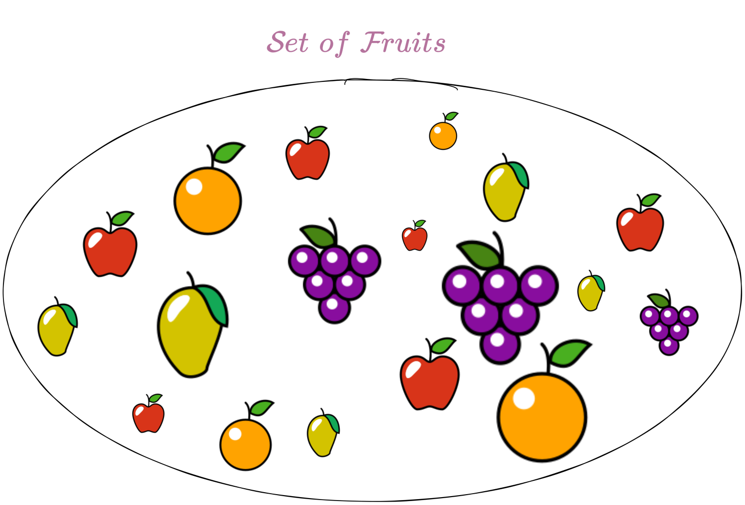
    Suppose we split this set of fruits into subsets based on the type of fruits as shown below. We can see that each subset is non-empty and every element of the set of fruits belongs to only one subset and consequently, the subsets are disjoint. Such a “partition” of the set of fruits based on the type of fruit can also be viewed as a set with an equivalence relation, namely, two fruits are equivalent if they are of the same type and each subset corresponds to an equivalence class.

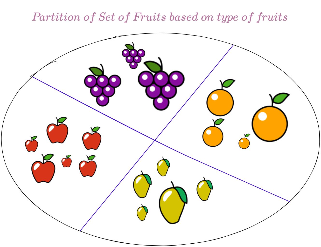
    We have illustrated through this example that a partition of a set is a grouping of its elements into non-empty subsets, in such a way that each element is included in exactly one subset.

    Every equivalence relation on a set defines a partition of this set and every partition defines an equivalence relation. A set equipped with an equivalence relation or a partition is also called a setoid.

    Definition

    A partition of a set X is a set of non-empty subsets of X such that every element x in X is in exactly one of these subsets i.e., the subsets are non-empty mutually disjoint sets.

    Equivalently, a family (or collection) of sets P is a partition of X if and only if all of the following conditions hold.

    • The family P does not contain the empty set i.e., \empty \not \in P.

    • The union of the sets in P is equal to X i.e., \bigcup_{A \in P} = X. The sets in P are said to exhaust or cover X.

    • The intersection of any two distinct sets in P is empty i.e., (\forall A, B \in P) \, A \neq B \implies A \cap B = \empty. The elements of P are said to be pairwise disjoint or mutually exclusive.

    The sets in P are called the blocks, parts or cells of the partition. If x \in X then we represent the cell containing x by [x] i.e., the cell in P which contains x is denoted by [x].

    Fundamental Theorem of Equivalence Relations

    For any equivalence relation on a set X, the set of its equivalence classes is a partition of X.

    Conversely, from any partition P of X, we can define an equivalence relation on X by setting x \sim y precisely when x \text{ and } y are in the same cell in P.

    Thus, the notions of equivalence relation and partition are essentially equivalent.

    Examples

    The following are some examples of a partition P of a set.

    • The empty set \empty has exactly one partition, namely, \empty i.e., if X = \empty, then P = \empty.

    • For any non-empty set X, P = \{X\} is a partition of X, called the trivial partition. Every singleton set has exactly one partition. For example, the singleton set X = \{x\} has exactly one partition, namely, P = \{X\} = \{\{x\}\}.

    • For any non-empty proper subset X of a set U, the set X together with its complement form a partition of U, namely, partition P = \{X, U \!\setminus\! X\}.

    • The set X = \{1, 2, 3\} has 5 possible partitions.

      (i) P = \{\{1\}, \{2\}, \{3\}\}

      (ii) P = \{\{1\}, \{2, 3\}\}

      (iii) P = \{\{1, 3\}, \{2\}\}

      (iv) P = \{\{1, 2\}, \{3\}\}

      (v) P = \{\{1, 2, 3\}\}

    The following are not partitions of the set X = \{1, 2, 3\} :

    • \{\{\}, \{1, 2\}, \{3\}\} is not a partition of any set because one of its elements is the empty set.

    • \{\{1, 2\}, \{2, 3\}\} is not a partition of any set because the element 2 is contained in more than one cell.

    • \{\{1\}, \{2\}\} is not a partition of the set X because none of its cells contains 3.
    Representative of an Equivalence Class

    Every element of an equivalence class characterizes the class, and may be used to represent it. When such an element is chosen, it is called the representative of the class.

    Sometimes, a particular element of an equivalence class is more naturally suited to represent the class as compared to all other elements of the class. Such a representative is called a canonical representative i.e., it denotes the standard way to represent the equivalence class.

    Definition of Canonical Form

    Given a set S of mathematical objects with an equivalence relation R on S, a canonical form is given by designating some mathematical objects of S to be in “canonical form”, such that every mathematical object under consideration is equivalent to exactly one mathematical object in canonical form.

    Therefore, the canonical forms in S represent the equivalence classes once and only once. To test whether two mathematical objects are equivalent, it then suffices to test equality on their canonical forms.

    Canonical forms are generally used to make operating with equivalence classes more effective. For example, in the case of the congruence modulo n equivalence relation on the set of integers \mathbb{Z}, each congruence class modulo n may be represented by any one of its members, although we usually represent each congruence class by the smallest nonnegative integer which belongs to that class since this is the remainder which results from division by n. Operations on classes are carried out by combining these representatives and then reducing the result to its remainder when it is divided by n.

    Examples of Equivalence Classes

    Let X be the set of all triangles and \sim, the equivalence relation “has the same area as”. Then, for every positive real number A, there will be an equivalence class of all triangles that have the area A.

    We have already shown that congruence modulo n is an equivalence relation on the set of integers.

    The congruence modulo \mathit{4} equivalence relation, R, on the set of integers \mathbb{Z} is defined as :

    R = \big\{(x, y) \,|\, x \in \mathbb{Z}, y \in \mathbb{Z}, x \equiv y \!\!\! \pmod{4} \big\}

    That is, x is equivalent to y if and only if they leave the same non-negative integer as remainder when divided by 4. This equivalence relation gives rise to exactly 4 equivalence classes, one class for each possible remainder when an integer is divided by 4.

    The 4 equivalence classes corresponding to the remainders 0, 1, 2 \text{ and } 3 are shown below :

    \begin{equation*} 
    \begin{split}
    [0] &= \{\dots, -12, -8, -4, 0, 4, 8, 12, \dots\}\\
    [1] &= \{\dots, -11, -7, -3, 1, 5, 9, 13, \dots\}\\
    [2] &= \{\dots, -10, -6, -2, 2, 6, 10, 14, \dots\}\\
    [3] &= \{\dots, -9, -5, -1, 3, 7, 11, 15, \dots\}\\
    \end{split}
    \end{equation*} 

    [0], [1], [2] \text{ and } [3] are the canonical representatives of the equivalence classes corresponding to remainders 0, 1, 2 \text{ and }3.

    The quotient set, i.e., the set of all equivalence classes of \mathbb{Z} with respect to the congruence modulo n equivalence relation, R, is denoted by \mathbb{Z}\, / 4\mathbb{Z} and is defined as

    \mathbb{Z}\, / 4\mathbb{Z} = \{[0], [1], [2], [3]\}
    Well-definedness under an Equivalence Relation

    Suppose \sim is an equivalence relation on set X. Given an element x \in X, the equivalence class of x is the set

    [x] = \{y \in X : x \sim y\}

    The element x is called the representative of the equivalence class [x] and any element of an equivalence class can serve as its representative.

    The set of all equivalence classes of X with respect to the equivalence relation \sim is denoted by X\!/\!\!\sim and defined as

    X\!/\!\!\sim \, := \{[x] : x \in X\}

    This set, X\!/\!\!\sim, is called the quotient set of X with respect to \sim.

    Since an equivalence class can have different representations, any function we define with X\!/\!\!\sim as its domain should map different representations of the same equivalence class to the same element in its codomain to be considered a well-defined function (or just a function).

    Let us illustrate this constraint on the definition of a function with a X\!/\!\!\sim as its domain through an example.

    Let us attempt to define a function, f : \mathbb{Z}/7\mathbb{Z} \rightarrow \mathbb{Z}, as f([x]) = x.

    We can see that

    f([0]) = 0, \,f([2]) = 2, \,f([7]) = 7

    and so on. But this definition poses a problem. Since 0 \equiv 7 \pmod{7}, it implies that [0] = [7]. That is, [0] \text{ and } [7] are the exact same element of the set \mathbb{Z}/7\mathbb{Z}. However, as per the “function” we have defined above, f([0]) \neq f([7]). This is a violation of the definition of a function. Hence, f is not a function i.e., f is not well-defined because it maps different representations of the same equivalence class to different elements in its codomain.

    Let us attempt to rectify this issue by defining another function with domain \mathbb{Z}/7\mathbb{Z}.

    Consider a function, f : \mathbb{Z}/7\mathbb{Z} \rightarrow \{0, 1, 2, 3, 4, 5, 6\}, defined as

    f([x]) = x \bmod 7

    where x \bmod 7 is the remainder, as in the Division Algorithm, when x is divided by 7. That is, x \bmod 7 denotes the unique integer r such that 0 \leq r < 7 and r \equiv x \pmod 7.

    Now,

    f([0]) = 0, \,f([2]) = 2, \,f([7]) = 0

    We have already shown that [0] = [7] and we can see that f([0]) = f([7]).

    If f([x]) is a well-defined function, then for any x \in \mathbb{Z}, f([x]) = f([x^\prime]) whenever x \equiv x^\prime \pmod{7}, i.e., the definition of f([x]) does not depend on the choice of the representative x of the equivalence class.

    Let us verify whether f is a well-defined function i.e., whether f([x]) = f([x^\prime]) whenever x \equiv x^\prime \pmod{7}.

    Let us assume that there exist some integers x, x^\prime \in X such that x \equiv x^\prime \pmod{7}.

    By definition of congruence modulo n, n \,|\, (x - x^\prime) i.e., there exists some integer k \in \mathbb{Z} such that,

    x - x^\prime = kn

    Substituting n = 7 in the above equation,

    x = x^\prime + 7k

    Applying the Division Algorithm to x^\prime \text{ and } 7, yields unique integers q \text{ and } r such that,

    x^\prime = 7q + r

    where r \in \{0, 1, 2, 3, 4, 5, 6\}.

    Hence, f([x^\prime]) = r by definition of f.

    Combining the above two equations, we get

    x = 7q + r + 7k = 7(q+k) + r

    Therefore, f([x]) = r.

    We have shown that f([x]) = f([x^\prime]) whenever x \equiv x^\prime \pmod{7} i.e., f is well-defined.

    Well-defined Function with domain as Quotient Set

    Through the above example we have shown that in order to have a well-defined function, f : X\!/\!\!\sim \,\rightarrow Y\!, it must be the case that f([x]) = f([x^\prime]) whenever x \sim x^\prime for any x, x^\prime \in X.

    A typical argument for verifying that a function, f : X\!/\!\!\sim \,\rightarrow Y\!, is well defined is as follows.

    We take some arbitrary elements x, x^\prime \in X such that x \sim x^\prime and show that the proposed expressions for f([x]) \text{ and } f([x^\prime]) result in the same element in Y. In such a case, we can say that the proposed expression for f([x]) depends only on the equivalence class of x and not on the representative x itself and hence, the function, f, is well-defined.

    Theorem

    Let \sim be an equivalence relation on X. The necessary and sufficient condition for the binary relation, f : X\!/\!\!\sim \,\rightarrow Y\!, to be a (well-defined) function is that f([x]) = f([x^\prime]) whenever x \sim x^\prime for any x, x^\prime \in X.

    Suppose f : X\!/\!\!\sim \,\rightarrow Y\!, is a binary relation such that f([x]) = f([x^\prime]) whenever x \sim x^\prime for any x, x^\prime \in X. We will prove that f is a (well-defined) function.

    The binary relation, f, over sets X\!/\!\!\sim \text{ and } Y, that is, f \subseteq (X\!/\!\!\sim) \times Y is defined as

    f = \{([x], y) : [x] \in X\!/\!\!\sim \wedge \,\, y \in Y\}

    We will prove that the binary relation f over sets X\!/\!\!\sim \text{ and } Y is a function.

    From the definition of f we can see that for every [x] \in X\!/\!\!\sim there is a y \in Y such that ([x], y) \in f.

    For the uniqueness assertion, suppose that ([x], y) \in f \text{ and } ([x^\prime], y^\prime) \in f such that [x] = [x^\prime].

    Since [x] = [x^\prime] it follows that x \in [x^\prime] and hence, by definition of equivalence class x \sim x^\prime.

    Therefore, f([x]) = f([x^\prime]) and since y = f([x]) \text{ and } y^\prime = f([x^\prime]), it implies that y = y^\prime.

    Therefore, by definition of a function, the binary relation f over sets X\!/\!\!\sim \text{ and } Y is a function.

    Suppose f : X\!/\!\!\sim \,\rightarrow Y is a well-defined function. We have to prove that f([x]) = f([x^\prime]) whenever x \sim x^\prime for any x, x^\prime \in X.

    Suppose x \sim x^\prime for some arbitrary x, x^\prime \in X. Then, by definition of equivalence class, [x] = [x^\prime].

    Since f : X\!/\!\!\sim \,\rightarrow Y is a well-defined function, whenever [x] = [x^\prime] it must be the case that f([x]) = f([x^\prime]).

    Hence, we have proved the theorem.

    Ternary Relation

    Suppose we have a set of men, M, a set of women, W and a set of children, C. A possible relation, R, between these sets could be defined as “x \text{ is the child of } y \text{ and } z” . This would result in R being a set of 3\text{-tuples} also called triples such that each triple in R will have a child from set C associated with a father from set M and a mother from set W.

    The set R could therefore be viewed as a subset of the Cartesian product of the three sets C, M \text{ and }W denoted by C \times M \times W, which is the set of all ordered triples (c, m, w) where c belongs to set C, m belongs to set M and w belongs to set W. Therefore, R \subseteq C \times M \times W.

    A ternary relation, R, over the sets X, Y \text{and } Z is a new set of ordered triples (x, y, z) consisting of elements x from X, y from Y and z from Z. That is, elements x, y \text{ and } z are related if and only if the triple (x, y, z) belongs to the set of ordered triples that defines the ternary relation.

    It should be noted that the ternary relation, R, over the sets X, Y \text{and } Z can be defined solely as a set of ordered triples (x, y, z) where x \in X, y \in Y and z \in Z, without specifying the underlying relationship between x, y \text{ and } z.

    Definition

    A ternary relation R over sets X_1, X_2 \text{ and } X_3 is a subset of the Cartesian product X_1 \times X_2 \times X_3.
    That is, R \subseteq X_1 \times X_2 \times X_3.

    The set X_i is called the ith domain of R i.e., the sets X_1, X_2 \text{ and } X_3 are the first, second and third domains, respectively, of R.

    The statement (x_1, x_2, x_3) \in R reads “x_1, x_2, x_3 are R-related” and are denoted using prefix notation by Rx_1x_2x_3 and using postfix notation by x_1x_2x_3R. (A prefix notation is a type of mathematical notation in which the operators precede their operands, while in the postfix notation the operators follow their operands.)

    When X_1 = X_2 = X_3, a ternary relation is called a homogeneous relation or endorelation.

    In a ternary relation, the ordering of elements is important. That is, if x_1 \neq x_2 \neq x_3 then Rx_2x_3x_1 can be true or false independently of Rx_1x_2x_3. For example, 16 is divisible by 2 \text{ and } 4 but 2 is not divisible by 4 \text{ and } 16. Therefore, (16, 2, 4) \neq (2, 4, 16).

    Types of Ternary Relations

    The following are some types of ternary relations we will encounter during our study of mathematics.

    Binary Function

    A binary function, denoted by f, is a special type of ternary relation over sets X, Y \text{ and } Z that satisfies the following conditions :

    • For every x \in X \text{ and } y \in Y there exists z \in Z such that (x, y, z) \in f

    • (x, y, z) \in f \text{ and } (x, y, z^\prime) \in f imply that z = z^\prime

    We usually denote (x, y, z) \in f as f(x, y) = z.

    Also, since f is a ternary relation over sets X, Y \text{ and } Z it is a subset of the Cartesian product X \times Y \times Z i.e., f \subseteq X \times Y \times Z which is usually written as f : X \times Y \rightarrow Z, where X \times Y is the Cartesian product of X \text{ and } Y.

    For example, if \mathbb{Z} is the set of integers, \mathbb{Z}^+ is the set of positive integers and \mathbb{Q} is the set of rational numbers, then division is a binary function f : \mathbb{Z} \times \mathbb{Z}^+ \rightarrow \mathbb{Q}. (A rational number is any number that can be written in the form \dfrac{p}{q}, where p is an integer and q is a nonzero integer.)

    Binary Operation

    The binary operation, denoted by f, on the set X is a binary function over the set X.

    Since f is a homogeneous ternary relation over the set X, it is a subset of the Cartesian product X \times X \times X i.e., f \subseteq X \times X \times X which is usually written as f : X \times X \rightarrow X, where X \times X is the Cartesian product of X \text{ and } X.

    For example, the binary function + : \mathbb{Z} \times \mathbb{Z} \rightarrow \mathbb{Z} over the set of integers \mathbb{Z} is a binary operation because the sum of two integers is an integer.

    The element +(x, y) \in \mathbb{Z} is usually written as x + y.

    Mathematical Structure

    A mathematical structure is a non-empty set of mathematical objects, along with a specified collection of relations and functions defined on those objects, and a set of distinguished constants that are elements of that set. These components are determined by an irreducible set of axioms that function as the generative rules defining the permissible operations and the resultant relationships within the structure.

    A common way to represent a mathematical structure is as a tuple (Set, Operations/Functions, Relations, Constants).

    Note: While the most significant and deeply studied mathematical structures are governed by such axiomatic foundations, it is conceivable to consider mathematical structures in a broader sense where the specified components might not be explicitly determined by a formal and irreducible set of axioms. However, the power and utility of mathematical structures in building consistent and coherent theories often arise from their axiomatic underpinnings.

    Examples

    The Structure defined by Second-Order Peano Axioms

    The Peano axioms define a fundamental mathematical structure (\mathbb{N}_0, S, 0) involving:

    • A non-empty set of objects: The set of natural numbers, \mathbb{N}_0 = \{0, 1, 2, 3, \dots\}.

    • A distinguished constant: The natural number 0 \in \mathbb{N}_0.

    • A function: The successor function S : \mathbb{N}_0 \rightarrow \mathbb{N}_0, where S(n) is intuitively the next natural number after n in the sequence of natural numbers. This function defines a fundamental operation on the natural numbers.

    • Relations (defined by the axioms themselves): The Peano axioms themselves define crucial relations and properties within this structure:
      • Equality (=): Assumed as a fundamental logical relation.

      • Injectivity of the Successor Function: \forall m, n \in \mathbb{N}_0, (S(m) = S(n) \implies m = n). This defines a specific property of the successor function as a relation between natural numbers and their successors.

      • 0 is not a Successor: \forall n \in \mathbb{N}_0, (S(n) \neq 0). This defines a relationship between 0 and the range of the successor function.

      • The Induction Axiom (Second-Order): This axiom ensures the minimality of the set of natural numbers i.e., the set \mathbb{N}_0 consists of only the standard natural numbers that we know of and no other extraneous elements.

        This powerful axiom provides a method for proving statements about the entire set of natural numbers. It states that if a subset T \text{ of } \mathbb{N}_0 contains 0, and if for every n \text{ in } T, its successor S(n) is also in T, then T must be the set of natural numbers i.e., T = \mathbb{N}_0. In essence, if a property holds for 0 and is preserved by the successor function, it holds for all natural numbers.

    For a more detailed explanation of the Peano axioms and the structure they define, you can refer here.

    The Structure of the Real Numbers

    Consider the set of real numbers, \mathbb{R}. We can define a mathematical structure (\mathbb{R}, +, \times, <, 0, 1) on this set by including:

    • A non-empty set of objects: The set of real numbers, \mathbb{R}.

    • Relations: The order relation “<” (less than), which is a binary relation on \mathbb{R}.

    • Functions: The binary operations of addition “+” and multiplication “\times", which are functions from \mathbb{R} \times \mathbb{R} to \mathbb{R}.

    • Distinguished constants: 0 (the additive identity element in \mathbb{R} i.e., a + 0 = a, for any real number a) and 1 (the multiplicative identity element in \mathbb{R} i.e., a \times 1 = a, for any real number a).

    The operations and the order relation in this structure are determined by a fundamental set of axioms, including the field axioms (defining the properties of addition and multiplication) and the order axioms (defining the properties of the “less than” relation). Crucially, the real numbers are also characterized by the completeness axiom (often stated as the least upper bound property or Dedekind completeness), which ensures that every non-empty subset of \mathbb{R} that is bounded above has a least upper bound within \mathbb{R}. This axiom distinguishes the real numbers from the rational numbers, which do not satisfy it.

    Examples of Other Mathematical Structures

    Beyond these examples, the concept of a mathematical structure provides a unifying framework across diverse areas of mathematics. In mathematics, many specific types of structures are studied in detail, each with its own defining axioms and properties, such as groups (equipped with a single associative binary operation, an identity element, and inverses), rings (with two binary operations satisfying certain axioms), fields (which are commutative rings with multiplicative inverses for non-zero elements), and topological spaces (where the notion of “nearness” is formalized).

    Isomorphism

    A fundamental idea in the study of mathematical structures is that of isomorphism. Two mathematical structures are said to be isomorphic if they are of the same type (i.e., they satisfy the same defining axioms and have corresponding basic components) and there exists a structure-preserving bijection between their underlying sets. Intuitively, isomorphic structures are considered to be essentially the same, differing only in the names of their elements.

    Model Theory

    The formal framework for studying mathematical structures, including their types and isomorphisms, is provided by model theory, a branch of mathematical logic that rigorously investigates the relationship between formal axiomatic theories and their interpretations, known as models. These models are, in essence, the mathematical structures that satisfy the axioms of a given theory, providing a deep and abstract perspective on the foundations of mathematics.

    To illustrate this connection, consider Peano’s Axioms, which form a formal theory about the natural numbers. The formal language of Peano Arithmetic uses abstract symbols to represent the natural numbers, including the constant symbol 0, the unary function symbol S, variables like n, m, x, y, and logical symbols such as \forall, \exists, \text{ and } =. The standard structure of the natural numbers (\mathbb{N}_0​, S, 0), where \mathbb{N}_0​ is the set of natural numbers, S is the successor function, and 0 is zero, serves as a model for these axioms because the model gives these symbols concrete meaning. For example, the constant symbol “0" refers to the number zero itself, the function symbol “S" refers to the successor function, the symbols “\forall " and “\exists " mean “for all” and “there exists” when quantifying over the natural numbers, and the symbol “=” represents the actual equality relationship between natural numbers. Under this interpretation, all the axioms of Peano Arithmetic are true in the structure (\mathbb{N}_0​, S, 0).

    Categories
    cryptography mathematics

    Definition of Cipher

    authored by Premmi and Beguène

    A cipher defines the mechanism through which a message is transformed into a ciphertext using a key such that only the entities sharing this key could use it to decrypt the ciphertext and recover the message.

    A cipher, \mathcal{E}, comprises of a pair of functions, namely, the encryption and decryption functions. That is,

    \mathcal{E} = (E, D)

    where E denotes the encryption function and D, the decryption function.

    The encryption function, E, takes as input a key, k, and a message, m and produces as output a ciphertext, c. That is,

    c = E(k, m)

    and we refer to ciphertext, c, as the encryption of m under k.

    The decryption function, D, takes as input a key, k, and a ciphertext, c and produces as output a message, m. That is,

    m = D(k,c)

    and we refer to message, m, as the decryption of c under k.

    Since it must be possible to recover m given c \text{ and } k, the cipher must satisfy the following correctness property.

    For every key in the key space and every message in the message space,

    D(k, \,E(k, m)\,) = m

    An alternate way to write the encryption and decryption functions are as follows:

    \begin{equation*} 
    \begin{split}
    E &: \mathcal{K} \,{\small \times}\, \mathcal{M} \rightarrow \mathcal{C} \, \&\\ 
    D &: \mathcal{K} \,{\small \times}\, \mathcal{C} \rightarrow \mathcal{M} \\
    \end{split}
    \end{equation*}

    where \mathcal{K} denotes the set of all keys i.e., the key space, \mathcal{M} the set of all messages i.e., the message space and \mathcal{C} the set of all ciphertexts i.e., the ciphertext space.

    Henceforth, we will refer to the cipher, \mathcal{E}, as being defined over (\mathcal{K,\, M,\, C}).

    Computers process information which they receive in the form of input sequences. An input sequence is a finite sequence of symbols from some alphabet \mathit{A}. Since the most basic way of transmitting information is to code it into strings of 0\text{s and } 1\text{s}, such as 0010101, 1011001, etc., the alphabet \mathit{A} consists of only the two symbols, namely, 0 \text{ and } 1, i.e., \mathit{A} = \{0, 1\}.

    Such strings of 0\text{s and } 1\text{s} are called binary words, and the number of 0\text{s} and 1\text{s} in any binary word is called its length. That is, a binary word of length n is a string of n binary digits (a digit is either a 0 \text{ or } 1) or bits. Output sequences are defined in the same way as input sequences. The set of all sequences of symbols in this alphabet A of length L is denoted by \mathit{A} = \{0, 1\}^L.

    Hence, the keys, the messages and the ciphertexts are coded in the computers as sequences of bits.

    The key space \mathcal{K}, which is the set of all possible keys, each of length L, is represented as \mathcal{K} := \{0, 1\}^L. Similarly, \mathcal{M} := \{0, 1\}^L and \mathcal{C} := \{0, 1\}^L, represent the message space and the ciphertext space, where each message or ciphertext is a binary word of length L.

    We will also assume that \mathcal{K,\, M} \text{ and } \mathcal{C} are finite sets.

    Categories
    cryptography mathematics

    Perfect Secrecy

    authored by Premmi and Beguène

    Prerequisite : Probability Primer

    Follow up to : What is Security?

    Now that we have defined a secrecy system and discussed how to evaluate it, let us construct one based on the first and most important criterion, namely, a secrecy system that optimizes for secrecy i.e., a system that provides maximum secrecy. Such a secrecy system is called a perfectly secure system.

    Perfect Secrecy

    How can a secrecy system provide maximum secrecy?

    A secrecy system which is perfectly secure i.e., one which is maximally secure would provide no information about any of the messages it enciphers even if an adversary has unlimited time and computing resources to analyze any number of ciphertexts enciphered by the system.

    Now that we have agreed on the defining characteristic of a perfectly secure secrecy system, let us translate this characteristic into mathematics and analyze the properties of such a secrecy system.

    Let us assume that the possible messages m_0, m_1, \ldots, m_{n-1} (where n is the number of possible messages) are finite in number and their corresponding a priori probabilities are P(m_0), P(m_1), \ldots, P(m_{n-1}) and that these messages are enciphered into possible ciphertexts c_0, c_1, \ldots, c_{m-1} (where m is the number of possible ciphertexts) by

    c = T_i\,m

    where T_i is the transformation applied to message m to produce ciphertext c. The index i corresponds to the particular key being used.

    The adversary intercepts a particular ciphertext c and can then calculate, in principle at least, the a posteriori probabilities, P(M = m\,|\, C = c) for the various messages, where P(M = m\,|\, C = c) denotes the a posteriori probability of message m if ciphertext c is intercepted. Here M denotes the random variable defined on the message space (set of possible messages) and C, the random variable defined on the ciphertext space (set of possible ciphertexts).

    How can a ciphertext reveal (or leak) no information about the message it represents?

    Suppose an adversary with unlimited time and computing resources intercepts a ciphertext and constructs the distribution of the a posteriori probabilities of the various messages the ciphertext could decrypt to. In order for the adversary to gain no information from this distribution, it should be one of minimum information or equivalently, maximum entropy. Since the uniform distribution is the maximum entropy distribution among all discrete distributions, the distribution of a posteriori probabilities, namely, P(M = m\,|\, C = c) for various messages, should be uniform. Therefore, under this distribution, an intercepted ciphertext is equally likely to represent any of the possible messages. Hence, the adversary is forced to use his a priori knowledge of the message distribution, namely, P(M = m), to decipher the ciphertext since the intercepted ciphertext is equally likely to be the representation of any message in the message space and consequently, provides no information about which particular message it represents.

    Mathematically, we can represent this by the equation, P(M = m\,|\, C = c) = P(M = m).

    It should be noted that since a message is not picked at random but depends on the information a person wants to communicate, it has low entropy. Hence, a ciphertext can be viewed as the result of a transformation of a low entropy (high information) message into one of high entropy (low information). Hence, P(M = m\,|\, C = c) is uniform for various messages, though, the distribution of messages, P(M = m) is very rarely uniform.

    Definition

    Perfect secrecy is defined by the condition that for every ciphertext c, the a posteriori probabilities of the various messages representing this ciphertext are equal to the a priori probabilities of the same messages.That is,

    P(M = m\,|\, C = c) = P(M = m)

    for all m and c.

    This equation implies that the random variables M \text{ and } C are independent i.e., the message and ciphertext distributions are independent which is a consequence of the message leaking no information to the ciphertext and hence the adversary gaining no information from the intercepted ciphertext.

    Before we proceed further the above equation requires some clarification. This equation does not mean that the a posteriori probabilities of the various messages representing the ciphertext c, namely, P(M = m\,|\, C = c), are equal to the a priori probabilities of the messages, namely, P(M = m). On the contrary, it means that since the a posteriori probabilities, P(M = m\,|\, C = c), give no information about the particular message that was encrypted by the ciphertext, the adversary is forced to use his knowledge of the a priori probabilities of the various messages, namely, P(M = m), to guess the message that the intercepted ciphertext represents.

    Necessary and Sufficient Condition for Perfect Secrecy

    How do we prove that a secrecy system is perfectly secure? Based on our discussion, let us now formulate a necessary and sufficient condition for perfect secrecy. A secrecy system is perfectly secure only if it satisfies this condition, otherwise it is not perfectly secure.

    A necessary and sufficient condition for perfect secrecy can be found as follows.

    According to Bayes’ theorem, for discrete random variables X \text{ and } Y, we have

    P(Y = y\,|\,X = x) = \frac{P(Y = y)\, P(X = x \,|\,Y = y)}{P(X = x)}.

    Hence, by Bayes’ theorem,

    \begin{equation*} 
    \begin{split}
    P(M = m\,|\,C = c) &= \frac{P(M = m)\, P(C = c \,|\,M = m)}{P(C = c)} \\
    \text{where,} \quad \quad \quad \quad \quad \,\,\\
    P(M = m) &= \textit{a priori } \text{probability of message } m, \\
    P(C = c\,|\,M = m) &= \text{conditional probability of ciphertext \textit{c} if message \textit{m} is chosen} \\ 
    &\quad \,\,\, \text{i.e., the sum of the probabilities of all keys that produce ciphertext \textit{c} from message \textit{m},}  \\
    P(C = c) &= \text{the probability of obtaining ciphertext \textit{c} from any cause,} \\
    P(M = m\,|\,C = c) &= \textit{a posteriori \text{probability of message \textit{m} if ciphertext \textit{c} is intercepted}}.
    \end{split}
    \end{equation*} 

    We have already discussed that for perfect secrecy to hold,

    P(M = m\,|\,C = c) = P(M = m)

    for all c \text{ and all } m.

    Hence, either P(M = m) = 0, in which case P(M = m\,|\,C = c) = 0 or

    \frac{P(C = c \,|\,M = m)}{P(C = c)} = 1

    which implies,

    P(C = c \,|\,M = m) = P(C = c)

    for every m \text{ and } c.

    We exclude the solution P(M = m) = 0 because we want the condition for perfect secrecy, P(M = m\,|\,C = c) = P(M = m), to hold good independent of the value of P(M = m).

    For perfect secrecy to hold, it must be the case that

    P(M = m \,|\,C = c) = P(M = m)

    for all c \text{ and all } m.

    If

    P(C = c \,|\,M = m) = P(C = c) \neq 0

    for every m \text{ and } c, then

    P(M = m \,|\,C = c) = P(M = m)

    for all c \text{ and all } m and hence we have perfect secrecy.

    It should be noted that the equation P(C = c \,|\,M = m) = P(C = c) is of more interest to the designer of a perfect secrecy system than a cryptanalyst, while P(M = m \,|\,C = c) = P(M = m) is of more interest to a cryptanalyst.

    Therefore, we have the following result:

    A necessary and sufficient condition for perfect secrecy is that

    P(C = c \,|\,M = m) = P(C = c)

    for all m \text{ and } c; i.e., random variables M \text{ and } C are independent. This implies that the message and the ciphertext distributions are independent of each other.

    Design Constraints on a Perfect Secrecy System

    In order to construct a perfect secrecy system, we need to understand the constraints imposed by this equation on the design of such a system.

    So what are the consequences of this equation?

    Since M \text{ and } C are independent, it implies that the choice of a particular message m does not affect the probability of obtaining a particular ciphertext c. Therefore, every message m in the message space M should represent (or encipher to) a particular ciphertext c in the ciphertext space C with equal probability. This conclusion agrees with the above equation. Since,

    \begin{align*}
    P(C = c \,|\,M = m_0) &= P(C = c) \,\&\\
    P(C = c \,|\,M = m_1) &= P(C = c) \,\&\\
    &\vdots \\
    P(C = c \,|\,M = m_{n-1}) &= P(C = c) \\
    \end{align*}

    it follows that,

    P(C = c \,|\,M = m_0) = P(C = c \,|\,M = m_1) = \cdots = P(C = c \,|\,M = m_{n-1})

    for all c \in C and all m_i \in M, where i denotes the index of the message and takes values from 0 \text{ to } n-1. Here n is the number of messages in the message space M.

    Since the transformation of a message into a ciphertext corresponds to enciphering with a key, the above equation implies that the total probability of all keys that transform a message m_i into a given ciphertext c is equal to that of all keys transforming message m_j into the same ciphertext c, for all c, m_i \text{ and } m_j. Here i \text{ and }j denote the index of a message and take values from 0 \text{ to } n-1.

    This is illustrated below. Here r is the total probability of all the keys that transform any message m_i to a ciphertext c.

    It should be noted that only the total probability of all the keys transforming a message to a ciphertext needs to be equal to that of all the keys transforming any other message to the same ciphertext. The number of keys transforming a message to a ciphertext need not be equal to the number of keys transforming another message to the same ciphertext. Also the keys need not be equally likely i.e., each key can have its own associated probability different from other keys.

    A key which enciphers a particular message m into a ciphertext c also deciphers c into the same message m. Hence, the total probability of all keys that transform a message m_i into a given ciphertext c is equal to that of all keys transforming the ciphertext c into the same message m_i, for all c \text{ and } m_i. That is, for every c \in C,

    \begin{align*}
    P(C = c \,|\,M = m_0) &= P(M = m_0 \,|\,C = c) \,\&\\
    P(C = c \,|\,M = m_1) &= P(M = m_1 \,|\,C = c) \,\&\\
    &\,\,\,\vdots \\
    P(C = c \,|\,M = m_{n-1}) &= P(M = m_{n-1} \,|\,C = c) \\
    \end{align*}

    We have already shown that,

    P(C = c \,|\,M = m_0) = P(C = c \,|\,M = m_1) = \cdots = P(C = c \,|\,M = m_{n-1})

    for all c \in C.

    Hence,

    P(M = m_0 \,|\,C = c) = P(M = m_1 \,|\,C = c) = \cdots = P(M = m_{n-1} \,|\,C = c)

    for all c \in C.

    This is illustrated below.

    This image has an empty alt attribute; its file name is PerfectSecrecyEquation_2-1-919x1024.png
    Distribution of Ciphertexts

    We will next discuss whether the equation for perfect secrecy constrains the distribution of the ciphertexts in anyway i.e., does it necessitate the ciphertexts to have a particular distribution?

    For perfect secrecy,

    P(C = c \,|\, M = m) = P(C = c) \neq 0

    for every c \in C \text{ and } m \in M.

    The following is the necessary and sufficient condition for perfect secrecy enumerated for every m \text{ and } c.

    \begin{align*}
    \small P(C = c_0 \,|\,M = m_0) &= \small P(C = c_0) = r_0 \,\,\& \quad \small P(C = c_1 \,|\,M = m_0) = \small P(C = c_1)  = r_1\,\,\& \quad \cdots \quad \small P(C = c_{t-1} \,|\,M = m_0) = \small P(C = c_{t-1})  = r_{t-1}\,\,\&\\
    \\
    \small P(C = c_0 \,|\,M = m_1) &= \small P(C = c_0) = r_0 \,\,\& \quad \small P(C = c_1 \,|\,M = m_1) = \small P(C = c_1)  = r_1\,\,\& \quad \cdots \quad \small P(C = c_{t-1} \,|\,M = m_1) = \small P(C = c_{t-1})  = r_{t-1}\,\,\&\\
    \\
    &\,\,\,\vdots \quad\quad\quad\quad\quad\quad\quad\quad\quad\quad\quad\quad\quad\quad\quad\quad\,\,\,\,\,\,\vdots \quad\quad\quad\quad\quad\quad\quad\quad\quad\quad\quad\quad\quad\quad\quad\quad\quad\quad\,\,\,\,\,\,\,\,\,\,\,\vdots\\
    \\
    \small P(C = c_0 \,|\,M = m_{n-1}) &= \small P(C = c_0) = r_0 \quad \quad \small P(C = c_1 \,|\,M = m_{n-1}) = \small P(C = c_1)  = r_1\quad  \cdots \quad\small P(C = c_{t-1} \,|\,M = m_{n-1}) = \small P(C = c_{t-1})  = r_{t-1} \\
    \end{align*}

    Here m is the number of messages in the message space and t is the number of ciphertexts in the ciphertext space.

    These sets of equations are illustrated below :

    We have already seen that a perfect secrecy system satisfies the following equation

    P(M = m \,|\, C= c) = P(M = m)

    for all c \text{ and } m.

    Hence,

    \begin{align*}
    P(M = m_0 \,|\, C= c_0) &= P(M = m_0) \,\& \\
    P(M = m_0 \,|\, C= c_1) &= P(M = m_0) \,\& \\
    &\,\,\,\vdots \\
    P(M = m_0 \,|\, C= c_{t-1}) &= P(M = m_0) \,\& \\
    \end{align*}

    Therefore,

    P(M = m_0 \,|\, C= c_0) = P(M = m_0 \,|\, C= c_1) = \cdots = P(M = m_0 \,|\, C= c_{t-1})

    We have already shown above that

    \begin{align*}
    P(C = c_0 \,|\,M = m_0) &= P(M = m_0 \,|\,C = c_0) \,\&\\
    P(C = c_1 \,|\,M = m_0) &= P(M = m_0 \,|\,C = c_1) \,\&\\
    &\,\,\,\vdots \\
    P(C = c_{t-1} \,|\,M = m_0) &= P(M = m_0 \,|\,C = c_{t-1}) \\
    \end{align*}

    Therefore,

    P(C = c_0 \,|\, M= m_0) = P(C = c_1 \,|\, M = m_0) = \cdots = P(C = c_{t-1} \,|\, M= m_0)

    The necessary and sufficient condition for perfect secrecy states that,

    \begin{align*}
    P(C = c_0 \,|\,M = m_0) &= P(C = c_0) \,\&\\
    P(C = c_1 \,|\,M = m_0) &= P(C = c_1) \,\&\\
    &\,\,\,\vdots \\
    P(C = c_{t-1} \,|\,M = m_0) &= P(C = c_{t-1}) \\
    \end{align*}

    Therefore,

    P(C = c_0) = P(C = c_1) = \cdots = P(C = c_{t-1})

    Hence in a perfectly secure system the ciphertext distribution is uniform.

    These relationships are illustrated below:

    Relationship between |K| and |C|

    For perfect secrecy,

    P(C = c \,|\, M = m) = P(C = c) \neq 0

    for every c \in C \text{ and } m \in M.

    We have already shown above that any message in the message space enciphers to any ciphertext in the ciphertext space with equal and non-zero probability i.e., the value of P(C = c \,|\, M = m) is non-zero and the same for any c \in C \text{ and } m \in M.

    The following is the enumeration of this result for every m \in M \text{ and } c \in C.

    \begin{align*}
    \small P(C = c_0 \,|\,M = m_0) &= \small P(C = c_0) = r \,\,\& \quad \small P(C = c_1 \,|\,M = m_0) = \small P(C = c_1)  = r\,\,\& \quad \cdots \quad \small P(C = c_{t-1} \,|\,M = m_0) = \small P(C = c_{t-1})  = r\,\,\&\\
    \\
    \small P(C = c_0 \,|\,M = m_1) &= \small P(C = c_0) = r \,\,\& \quad \small P(C = c_1 \,|\,M = m_1) = \small P(C = c_1)  = r\,\,\& \quad \cdots \quad \small P(C = c_{t-1} \,|\,M = m_1) = \small P(C = c_{t-1})  = r\,\,\&\\
    \\
    &\,\,\,\vdots \quad\quad\quad\quad\quad\quad\quad\quad\quad\quad\quad\quad\quad\quad\quad\quad\,\,\,\,\,\,\vdots \quad\quad\quad\quad\quad\quad\quad\quad\quad\quad\quad\quad\quad\quad\quad\quad\quad\quad\,\,\,\,\,\,\,\,\,\,\,\vdots\\
    \\
    \small P(C = c_0 \,|\,M = m_{n-1}) &= \small P(C = c_0) = r \quad \quad \small P(C = c_1 \,|\,M = m_{n-1}) = \small P(C = c_1)  = r\quad  \cdots \quad\small P(C = c_{t-1} \,|\,M = m_{n-1}) = \small P(C = c_{t-1})  = r \\
    \end{align*}

    There are n messages in the message space and t ciphertexts in the ciphertext space.

    Below is an illustration of this result i.e., every message in the message space enciphering to every ciphertext in the ciphertext space with equal and non-zero probability, r.

    Since P(C = c \,|\, M = m) = P(C = c) \neq 0 for any c \in C \text{ and any } m \in M, it must be the case that there is at least one key transforming any m into any of the possible c\text{'s}.

    But all the keys transforming a particular message m into different c\text{'s} must be different so that given a message and a key unique encipherment is possible i.e., a key transforms a message into exactly one ciphertext. Therefore, the number of keys is at least equal to the number of ciphertexts, i.e., |K| \geq |C|.

    Since a key is first chosen and shared independent of the message that needs to be communicated, it means that a key should be able to encrypt any message in the message space. Hence every key in the key space can encipher any message in the message space.

    These two cases, |K| = |C| \text{ and } |K| > |C| are illustrated below.

    We have already proved that,

    P(C = c_0 \,|\, M= m_0) = P(C = c_1 \,|\, M = m_0) = P(C = c_2 \,|\, M= m_0)

    Hence, as shown in the illustration above, a particular message in the message space can be transformed into a ciphertext by one or more keys depending on the probability distribution of the keys such that the total probability of all keys that transform the message into a ciphertext is equal to that of all keys that transform the same message to any other ciphertext in the ciphertext space.

    We will next consider in some detail examples of perfect secrecy systems with |K| = |C| \text{ and } |K| > |C|.

    For the case |K| = |C|, we consider a perfect secrecy system with

    M = \{m_0, m_1, m_2\}, K = \{k_0, k_1, k_2\} \text{ and } C = \{c_0, c_1, c_2\}, as shown below.

    Since the transformation of a message into a ciphertext corresponds to enciphering with a particular key, the probability of a message resulting in a particular ciphertext equals the sum of probabilities of all keys that transform the message into that ciphertext (since given those keys, a message results in a particular ciphertext with probability 1, i.e., P(C = c \,|\, M = m, K = k) = 1 \,\forall\, \{k : c = T_k\, m\} where T_k is the transformation applied to message \mathcal{m} to produce ciphertext \mathcal{c}. The index k corresponds to the particular key being used.)

    Expressed as an equation,

    P(C = c \,|\, M = m) = \sum_{k \,\in\, K} P(K = k)\, P(C = c \,|\, M = m, K = k) 
    

    In the above example,

    \begin{equation*} 
    \begin{split}
    P(C = c_0 \,|\, M = m_0) & = \sum_{k \,\in\, K} P(K = k)\, P(C = c_0 \,|\, M = m_0, K = k) \\
    & = P(K = k_0)\, P(C = c_0 \,|\, M = m_0, K = k_0) \\
    & \quad+ P(K = k_1)\, P(C = c_0 \,|\, M = m_0, K = k_1)\\
    & \quad + P(K = k_2)\, P(C = c_0 \,|\, M = m_0, K = k_2) \\
    & = P(K = k_0) \times 1 + P(K = k_1) \times 0 + P(K = k_2) \times 0 \\
    & = P(K = k_0)
    \end{split}
    \end{equation*} 

    Since P(C = c_0 \,|\, M = m_0) = r, P(K = k_0) =r. Similarly, P(K = k_1) =r \text{ and } P(K = k_2)=r.

    Therefore,

    P(K = k_0) = P(K = k_1)=P(K = k_2)

    i.e., when |K| = |C|, the distribution of keys is uniform.

    Since P(C = c_0 \,|\, M= m_0) = P(C = c_1 \,|\, M = m_0) = P(C = c_2 \,|\, M= m_0) = r, i.e., the total probability of all keys transforming the message to a particular ciphertext equals that of all keys transforming the same message to any other ciphertext and there is only one key transforming the message to a particular ciphertext, each key has an equal probability, r, of being picked.

    For the case |K| > |C|,

    we consider a perfect secrecy system with M = \{m_0, m_1, m_2\}, K = \{k_0, k_1, k_2, k_3, k_4\} \text{ and } C = \{c_0, c_1, c_2\}, as shown below.

    For this perfect secrecy system,

    \begin{equation*} 
    \begin{split}
    P(C = c_0 \,|\, M = m_0) & = \sum_{k \,\in\, K} P(K = k)\, P(C = c_0 \,|\, M = m_0, K = k) \\
    & = P(K = k_0)\, P(C = c_0 \,|\, M = m_0, K = k_0) \\
    & \quad+ P(K = k_1)\, P(C = c_0 \,|\, M = m_0, K = k_1)\\
    & \quad + P(K = k_2)\, P(C = c_0 \,|\, M = m_0, K = k_2) \\
    & \quad + P(K = k_3)\, P(C = c_0 \,|\, M = m_0, K = k_3) \\
    & \quad + P(K = k_4)\, P(C = c_0 \,|\, M = m_0, K = k_4) \\
    & = P(K = k_0) \times 1 + P(K = k_1) \times 0 + P(K = k_2) \times 1 + P(K = k_3) \times 0 + P(K = k_4) \times 0\\
    & = P(K = k_0) + P(K = k_2) \\
    \end{split}
    \end{equation*} 

    Since P(C = c_0 \,|\, M = m_0) = r,

    P(K = k_0) + P(K = k_2) = r

    Similarly,

    \begin{equation*} 
    \begin{split}
    P(K = k_1) + P(K = k_3) &= r \,\&\\
    P(K = k_4) &= r \\
    \end{split}
    \end{equation*} 

    In this perfect secrecy system, each message can be transformed into a particular ciphertext by either one or two keys. Since a message can be enciphered by every key in the key space, each key has a non-zero probability of being chosen and as can be seen from the above equations, the distribution of keys is non-uniform.

    This perfect secrecy system with one possible probability distribution of keys is shown below.

    Here,

    \begin{align*}
    P(K = k_0) &= P(K = k_2) = \frac{1}{2}r \\
    P(K = k_1) &= \frac{1}{3}r \\
    P(K = k_3) &= \frac{2}{3}r \\
    P(K = k_4) &= r \\
    \end{align*}

    Since by the axiom of probability,

    P(K = k_0) + P(K = k_1) + P(K = k_2) + P(K = k_3) + P(K = k_4) = 1 
    

    it follows that,

    \begin{align*}
    \frac{1}{2}r + \frac{1}{3}r + \frac{1}{2}r + \frac{2}{3}r + r &= 1 \\
    3r &= 1 \\
    r &= \frac{1}{3} \\
    \end{align*}

    Hence,

    \begin{align*}
    P(K = k_0) &= P(K = k_2) = \frac{1}{2}r = \frac{1}{2} \times \frac{1}{3} = \frac{1}{6} \\
    P(K = k_1) &= \frac{1}{3}r = \frac{1}{3} \times \frac{1}{3} = \frac{1}{9} \\
    P(K = k_3) &= \frac{2}{3}r = \frac{2}{3} \times \frac{1}{3} = \frac{2}{9}\\
    P(K = k_4) &= r = \frac{1}{3} \\
    \end{align*}

    We can see that,

    P(C = c \,|\, M = m) = P(K = k_0) + P(K = k_2) = P(K = k_1) + P(K = k_3) = P(K = k_4) = r = \frac{1}{3}

    for every c \in C \text{ and } m \in M.

    The above equation shows that any message is transformed into any ciphertext by keys k_0 \text{ and } k_2 or keys k_1 \text{ and } k_3 or key k_4 with the same total probability r = \dfrac{1}{3}.

    There are more keys than ciphertexts (the key space consists of 5 keys, while the ciphertext space’s cardinality is 3) since a message is transformed into a ciphertext by one or two keys, such that P(C = c \,|\, M = m) = r for every c \in C \text{ and } m \in M and all the keys transforming a particular message m into different c \text{'s} must be different.

    Hence, |K| \geq |C|.

    Relationship between |K| and |M|

    We have already shown that any message in the message space enciphers to any ciphertext in the ciphertext space with equal and non-zero probability i.e., the value of P(C = c \,|\, M = m) is non-zero and the same for any c \in C \text{ and } m \in M.

    Below is an illustration of this result i.e., every message in the message space enciphering to every ciphertext in the ciphertext space with equal and non-zero probability, r.

    Since P(C = c \,|\, M = m) = P(C = c) \neq 0 for any c \in C \text{ and any } m \in M, it must be the case that there is at least one key transforming any m into any of the possible c\text{'s}.

    But all the keys transforming different messages into a particular ciphertext c must be different so that given a ciphertext and key unique decipherment is possible. Therefore, the number of keys is at least equal to the number of messages, i.e., |K| \geq |M|.

    It should also be noted that since a key is first chosen and shared independent of the message that needs to be communicated, it means that a key should be able to encrypt any message in the message space. Hence every key in the key space can encipher any message in the message space.

    These two cases, |K| = |M| \text{ and } |K| > |M| are illustrated below.

    Let us next consider two examples of perfect secrecy systems one with |K| = |M| \text{ and other with } |K| > |M|.

    For the case |K| = |M|, we consider a perfect secrecy system with

    M = \{m_0, m_1, m_2\}, K = \{k_0, k_1, k_2\} \text{ and } C = \{c_0, c_1, c_2\}, as shown below.

    As we have already shown in the case where |K| = |C|,

    \begin{equation*} 
    \begin{split}
    P(C = c_0 \,|\, M = m_0) & = \sum_{k \,\in\, K} P(K = k)\, P(C = c_0 \,|\, M = m_0, K = k) \\
    
    & = P(K = k_0)
    \end{split}
    \end{equation*}

    Similarly,

    P(C = c_0 \,|\, M = m_1) = P(K = k_1)

    and

    P(C = c_0 \,|\, M = m_2) = P(K = k_2)

    Since

    P(C = c_0 \,|\, M = m_0) = P(C = c_0 \,|\, M = m_1) = P(C = c_0 \,|\, M = m_2)

    it follows that,

    P(K = k_0) = P(K = k_1)=P(K = k_2)

    i.e., when |K| = |M|, the distribution of keys is uniform.

    Since P(C = c_0 \,|\, M= m_0) = P(C = c_1 \,|\, M = m_0) = P(C = c_2 \,|\, M= m_0) = r, i.e., the total probability of all keys transforming the message to a particular ciphertext equals that of all keys transforming the same message to any other ciphertext and there is only one key transforming the message to a particular ciphertext, each key has an equal probability, r, of being picked.

    For the case |K| > |M|,

    we consider a perfect secrecy system with M = \{m_0, m_1, m_2\}, K = \{k_0, k_1, k_2, k_3, k_4\} \text{ and } C = \{c_0, c_1, c_2\}, as shown below.

    As we have already shown in the case where |K| > |C|,

    P(C = c \,|\, M = m) = P(K = k_0) + P(K = k_2) = P(K = k_1) + P(K = k_3) = P(K = k_4) = r = \frac{1}{3}

    for every c \in C \text{ and } m \in M.

    The above equation shows that any message is transformed into any ciphertext by keys k_0 \text{ and } k_2 or keys k_1 \text{ and } k_3 or key k_4 with the same total probability r = \dfrac{1}{3}.

    In this perfect secrecy system there are more keys than messages (the key space consists of 5 keys, while the message space’s cardinality is 3) because a message is transformed into a ciphertext by one or two keys, such that P(C = c \,|\, M = m) = r for every c \in C \text{ and } m \in M and all the keys transforming different messages m into a particular ciphertext c must be different so that given a ciphertext and key unique decipherment is possible.

    Hence, |K| \geq |M|.

    Relationship between |C| and |M|

    Since any key in the key space enciphers every message in the message space to a different ciphertext such that given the ciphertext and key, unique decipherment is possible, there must be at least as many ciphertexts as there are messages i.e.,

    |C| \geq |M|

    We illustrate the two cases, namely, |C| = |M| \text{ and } |C| > |M| below.

    Below is the illustration of a perfect secrecy system with |C| = |M|, where the message space consists of 3 messages, the key space consists of 3 keys and the ciphertext space also consists of 3 ciphertexts. The keys are drawn from a uniform distribution and the probability of choosing a key is \dfrac{1}{3}, i.e., r = \dfrac{1}{3}.

    We can see that for any key in the key space there is a one-to-one correspondence between all the messages in the message space and all the ciphertexts in the ciphertext space.

    Next let us explore the case when |C| > |M|.

    From the two illustrations shown below depicting the cases |K| = |M| \text{ and } |K| > |M|, we can see that the entire key space is exhausted by all the messages that transform to a particular ciphertext i.e., every message in the message space transforms to a particular ciphertext through some permutation of the entire key space.

    From the illustration on the left, where |K| = |M|, we can see that some permutation of the entire key space i.e., K = \{k_0, k_1, k_2\} transforms the message space i.e., M = \{m_0, m_1, m_2\} into a particular ciphertext, c.

    Similarly, in the illustration on the right, where |K| > |M|, some permutation of the entire key space i.e., K = \{k_0, k_1, k_2, k_3, k_4\} transforms the message space i.e., M = \{m_0, m_1, m_2\} into a particular ciphertext, c.

    However, in some cases when |K| > |M|, depending on the probability distribution of the keys, only a subset of the key space is exhausted (used) when the message space is transformed to a particular ciphertext as explained below.

    Consider a perfect secrecy system where the key space consists of 4 keys, all equally likely and the message space consists of only 3 messages.

    In a perfect secrecy system, the probability that a message transforms to a particular ciphertext equals that of the message transforming to any other ciphertext in the ciphertext space. Since in this particular perfect secrecy system every key in the key space has an equal probability, r, of being picked, and every key in the key space can encipher any message in the message space, each key in the key space transforms a particular message into a unique ciphertext so that the probability of the message transforming to any ciphertext in the ciphertext space is the same and equals r. Hence, each of the 4 keys encipher a particular message into 4 different ciphertexts as shown below. Since each of the 3 messages in the message space are transformed into 4 different ciphertexts by 4 equally likely keys, in this case, |C| > |M|.

    Since there are only 3 messages and each key is equally likely, there is only one unique key that transforms each of those messages into a particular ciphertext. Hence here only 3 out of the 4 keys are used to transform the message space into a particular ciphertext i.e., the entire key space is not used to transform the message space into a ciphertext. In the example shown above only keys k_0, k_1 \text{ and } k_2 are used to transform the 3 messages m_0, m_1 \text{ and } m_2 into ciphertext c_0.

    Therefore, for every key in the key space, there is a one-to-one correspondence between all messages in the message space and some of the ciphertexts in the ciphertext space.

    This case of |C| > |M| is illustrated below. Since the keys are drawn from a uniform distribution and there are four keys, r = \dfrac{1}{4}.

    We can see from the above illustration that every message is enciphered by all the four keys (since a key should be able to encipher any message in the message space), but every ciphertext is not deciphered by all the keys (in fact only 3 keys decipher each ciphertext). So for any fixed key there is a one-to-one correspondence between all the messages in the message space, and some of the ciphertexts in the ciphertext space.

    For example, for the key k_0, there is a one-to-one correspondence between the messages m_0, m_1 \text{ and } m_2 and the ciphertexts c_0, c_3 \text{ and } c_2 i.e., a one-to-one correspondence between all the 3 messages in the message space and 3 out of the 4 ciphertexts in the ciphertext space. This is a consequence of |K| > |M| and each key being equally likely i.e., the key space having a uniform distribution (and also the total probability of each message transforming to a particular ciphertext requiring to equal that of every other message transforming to the same ciphertext).

    It should be noted that though all keys don’t decipher a particular ciphertext, a ciphertext still deciphers to every message in the message space with equal probability and also every message in the message space also enciphers to every ciphertext in the ciphertext space with equal probability. Hence perfect secrecy is still maintained.

    So far we have proved that,

    \begin{equation*} 
    \begin{split}
    |K|  & \geq |C| \\
    |K|  & \geq |M|  \text{ and} \\
    |C|  & \geq |M| \\
    \end{split}
    \end{equation*}

    It follows from the above inequalities that,

    |K|  \geq |C| \geq |M|

    As an aside, though we don’t need |K| \geq |M| to prove the above relationship, we needed it to prove |C| \geq |M|.

    Various kinds of Perfect Secrecy Systems

    Perfect Secrecy System with |K| > |C| > |M|

    By axiom of probability,

    \begin{equation*} 
    \begin{split}
    P(C = c_0 \,|\, M = m_0) + P(C = c_1 \,|\, M = m_0) + P(C = c_2 \,|\, M = m_0)&= 1 \\
    r + r + r &= 1\\
    3r &= 1 \\
    r &= \frac{1}{3}\\
    \end{split}
    \end{equation*}

    Also,

    \begin{equation*} 
    \begin{split}
    P(C = c) &= \sum_{m \,\in\, M} P(M = m)\, P(C = c \,|\, M = m) \\
    &=  \sum_{m \,\in\, M} P(M = m) \times r \\
    &= r \sum_{m \,\in\, M} P(M = m) \\
    &= r \\
    \end{split}
    \end{equation*}

    for every c \in C, since P(C = c \,|\, M = m) = r for every c \in C \text{ and } m \in M and by axiom of probability, \displaystyle \sum_{m \,\in\, M} P(M = m) = 1.

    Therefore,

    P(C = c \,|\, M = m) = P(C = c) = \frac{1}{3}

    for all c \in C \text{ and } m \in M.

    Also,

    \begin{equation*} 
    \begin{split}
    P(C = c_0 \,|\, M = m_0) & = \sum_{k \,\in\, K} P(K = k)\, P(C = c_0 \,|\, M = m_0, K = k) \\
    
    & = P(K = k_0)
    \end{split}
    \end{equation*}

    Similarly,

    P(C = c_1 \,|\, M = m_0) = P(K = k_1)

    and

    P(C = c_2 \,|\, M = m_0) = P(K = k_2) + P(K = k_3) 

    Therefore,

    P(K = k_0) = P(K = k_1) = r = \frac{1}{3}

    and

    P(K = k_2) = P(K = k_3) = \frac{1}{2}r = \frac{1}{6}

    In this perfect secrecy system, each message is transformed to a particular ciphertext by one or two keys.

    Also, for every key in the key space there is a one-to-one correspondence between all the messages in the message space and some of the ciphertexts in the ciphertext space. For example, for key k_0, there is a one-to-one correspondence between messages m_0 \text{ and } m_1 and ciphertexts c_0 \text{ and } c_1.

    The distribution of keys is non-uniform.

    Perfect Secrecy System with |K| > |C| = |M|

    By axiom of probability,

    \begin{equation*} 
    \begin{split}
    P(C = c_0 \,|\, M = m_0) + P(C = c_1 \,|\, M = m_0) &= 1 \\
    \frac{3}{2}r + \frac{3}{2}r &= 1\\
    3r &= 1 \\
    r &= \frac{1}{3}\\
    \end{split}
    \end{equation*}

    Also,

    \begin{equation*} 
    \begin{split}
    P(C = c) &= \sum_{m \,\in\, M} P(M = m)\, P(C = c \,|\, M = m) \\
    &=  \sum_{m \,\in\, M} P(M = m) \times \frac{3}{2}r \\
    &= \frac{3}{2}r \sum_{m \,\in\, M} P(M = m) \\
    &= \frac{3}{2}r \\
    \end{split}
    \end{equation*}

    for every c \in C, since P(C = c \,|\, M = m) = \dfrac{3}{2}r for every c \in C \text{ and } m \in M and by axiom of probability, \displaystyle \sum_{m \,\in\, M} P(M = m) = 1.

    Therefore,

    P(C = c \,|\, M = m) = P(C = c) = \frac{3}{2}r =\frac{1}{2}

    for all c \in C \text{ and } m \in M.

    Also,

    \begin{equation*} 
    \begin{split}
    P(C = c_0 \,|\, M = m_0) & = \sum_{k \,\in\, K} P(K = k)\, P(C = c_0 \,|\, M = m_0, K = k) \\
    
    & = P(K = k_0) + P(K = k_2) \\
    \end{split}
    \end{equation*}

    Similarly,

    P(C = c_1 \,|\, M = m_0) = P(K = k_1) + P(K = k_3) 

    As can be seen from the above illustration,

    P(K = k_0) = P(K = k_1) = r = \frac{1}{3}

    and

    P(K = k_2) = P(K = k_3) = \frac{1}{2}r = \frac{1}{6}

    In this perfect secrecy system, each message is transformed to a particular ciphertext by exactly two keys.

    Also, for every key in the key space there is a one-to-one correspondence between all the messages in the message space and all the ciphertexts in the ciphertext space.

    The distribution of keys is non-uniform.

    Perfect Secrecy System with |K| = |C| > |M|

    By axiom of probability,

    \begin{equation*} 
    \begin{split}
    P(C = c_0 \,|\, M = m_0) + P(C = c_1 \,|\, M = m_0) + P(C = c_2 \,|\, M = m_0) + P(C = c_3 \,|\, M = m_0)&= 1 \\
    r + r + r + r &= 1\\
    4r &= 1 \\
    r &= \frac{1}{4}\\
    \end{split}
    \end{equation*}

    Also,

    \begin{equation*} 
    \begin{split}
    P(C = c) &= \sum_{m \,\in\, M} P(M = m)\, P(C = c \,|\, M = m) \\
    &=  \sum_{m \,\in\, M} P(M = m) \times r \\
    &= r \sum_{m \,\in\, M} P(M = m) \\
    &= r \\
    \end{split}
    \end{equation*}

    for every c \in C, since P(C = c \,|\, M = m) = r for every c \in C \text{ and } m \in M and by axiom of probability, \displaystyle \sum_{m \,\in\, M} P(M = m) = 1.

    Therefore,

    P(C = c \,|\, M = m) = P(C = c) = \frac{1}{4}

    for all c \in C \text{ and } m \in M.

    Also,

    \begin{equation*} 
    \begin{split}
    P(C = c_0 \,|\, M = m_0) & = \sum_{k \,\in\, K} P(K = k)\, P(C = c_0 \,|\, M = m_0, K = k) \\
    
    & = P(K = k_0)
    \end{split}
    \end{equation*}

    Similarly,

    \begin{equation*} 
    \begin{split}
    P(C = c_1 \,|\, M = m_0) &= P(K = k_1), \\
    P(C = c_2 \,|\, M = m_0) &= P(K = k_2)\& \\
    P(C = c_3 \,|\, M = m_0)&= P(K = k_3) \\
    \end{split}
    \end{equation*}

    Therefore,

    P(K = k_0) = P(K = k_1) = P(K = k_2) = P(K = k_3) = r = \frac{1}{4}

    In this perfect secrecy system, each message is transformed to a particular ciphertext by exactly one key. Hence, the distribution of keys is uniform.

    Also, for every key in the key space there is a one-to-one correspondence between all the messages in the message space and some of the ciphertexts in the ciphertext space. For example, for key k_0, there is a one-to-one correspondence between messages m_0, m_1 \text{ and } m_2 and ciphertexts c_0, c_3 \text{ and } c_2.

    Perfect Secrecy System with |K| = |C| = |M|

    By axiom of probability,

    \begin{equation*} 
    \begin{split}
    P(C = c_0 \,|\, M = m_0) + P(C = c_1 \,|\, M = m_0) + P(C = c_2 \,|\, M = m_0) + P(C = c_3 \,|\, M = m_0)&= 1 \\
    r + r + r + r &= 1\\
    4r &= 1 \\
    r &= \frac{1}{4}\\
    \end{split}
    \end{equation*}

    Also,

    \begin{equation*} 
    \begin{split}
    P(C = c) &= \sum_{m \,\in\, M} P(M = m)\, P(C = c \,|\, M = m) \\
    &=  \sum_{m \,\in\, M} P(M = m) \times r \\
    &= r \sum_{m \,\in\, M} P(M = m) \\
    &= r \\
    \end{split}
    \end{equation*}

    for every c \in C, since P(C = c \,|\, M = m) = r for every c \in C \text{ and } m \in M and by axiom of probability, \displaystyle \sum_{m \,\in\, M} P(M = m) = 1.

    Therefore,

    P(C = c \,|\, M = m) = P(C = c) = \frac{1}{4}

    for all c \in C \text{ and } m \in M.

    Also,

    \begin{equation*} 
    \begin{split}
    P(C = c_0 \,|\, M = m_0) & = \sum_{k \,\in\, K} P(K = k)\, P(C = c_0 \,|\, M = m_0, K = k) \\
    
    & = P(K = k_0)
    \end{split}
    \end{equation*}

    Similarly,

    \begin{equation*} 
    \begin{split}
    P(C = c_1 \,|\, M = m_0) &= P(K = k_1), \\
    P(C = c_2 \,|\, M = m_0) &= P(K = k_2)\& \\
    P(C = c_3 \,|\, M = m_0)&= P(K = k_3) \\
    \end{split}
    \end{equation*}

    Therefore,

    P(K = k_0) = P(K = k_1) = P(K = k_2) = P(K = k_3) = r = \frac{1}{4}

    In this perfect secrecy system, each message is transformed to a particular ciphertext by exactly one key. Hence, the distribution of keys is uniform.

    Also, for every key in the key space there is a one-to-one correspondence between all the messages in the message space and all the ciphertexts in the ciphertext space. For example, for key k_0, there is a one-to-one correspondence between messages m_0, m_1, m_2 \text{ and } m_3 and ciphertexts c_0, c_3, c_2 \text{ and } c_1.

    Perfect secrecy systems in which the number of keys, the number of messages and the number of ciphertexts are all equal are characterized by the following properties :

    1. Every message in the message space is transformed to a particular ciphertext in the ciphertext space by exactly one key.
    2. All the keys in the key space are equally likely.

    Hence, from an implementation perspective the simplest (or easiest) possible perfect secrecy system to build is one in which the number of keys, the number of messages and the number of ciphertexts are all equal, i.e.,

    |K| = |C| = |M|

    Reusing keys makes a Perfect Secrecy System Insecure

    Since a perfect secrecy system transforms a message into a ciphertext in a deterministic way i.e., the same message will always generate the same ciphertext for the same key, as we have already discussed, reusing the key to encipher more than one message will make the prefect secrecy system insecure.

    The following example shows how a perfect secrecy system can become insecure if the same key is used to encipher more than one message.

    Suppose Maria decides to lives between Paris and Milan during the next 100 days. She will spend 80\% of her time in Paris and the remaining 20\% in Milan i.e., 80 days in Paris and 20 days in Milan. Also, in every 10 days period she will spend between 1 \text{ to } 3 days in Milan and the remaining days in Paris. She would like to communicate her location to Bob every single day in secrecy so that no one else knows her whereabouts. They use a simple perfect secrecy system as detailed below.

    Let us consider two scenarios, namely, one in which Maria shares a key with Bob only once and then reuses the same key to encipher her location and send it to Bob every time she communicates her location to him. In the other scenario, every time Maria wishes to communicate her location to Bob she picks a key at random from the key space and then encrypts the message (location) using that key. Let us analyze the security of the perfect secrecy system in both these scenarios.

    In the first scenario, Maria meets Bob before leaving for Paris and shares key k_1 with him. Over the next 100 days she will use this key to encrypt her communication with Bob.

    Following table shows her location for the first ten days, together with the ciphertext she sent to Bob each day to communicate her location to him encrypted using the shared key k_1.

    Suppose an eavesdropper intercepts the communication between Maria and Bob and observes the ciphertexts. He will see that 7 days the location was encrypted to c_1 and 3 days to c_0. Suppose he is aware of the probability distribution of the message space i.e., Maria spending majority of the time in Paris, then observing that c_1 occurs more frequently than c_0 he will rightly deduce that ciphertext c_1 is the encryption of Paris and c_0 of Milan. Hence without even knowing the encryption key, he will be able to decipher the message and hence know where Maria will be each day by intercepting the ciphertext alone, thereby making the secrecy system useless.

    Let us now consider an alternate scenario. Maria meets Bob each day and shares with him a key which she picks at random. Next day using this key, she encrypts her location and sends it to Bob and Bob meets her at that location.

    Following table shows her location for the first ten days, together with the ciphertext she sent to Bob each day to communicate her location to him encrypted using the shared key k_0 \text{ or } k_1 which she picked at random with equal probability.

    Suppose an eavesdropper observes the ciphertexts that Maria sends to Bob. He sees that on 6 days c_1 was sent and 4 days c_0 was sent. Since he is aware that Maria spends majority of her days in Paris, he assumes c_1 to be the encryption of Paris and c_0 Milan. Now suppose he decrypts under this assumption. Looking at the table, we can see that he will be right on days 1, 4, 7, 9 \text{ and } 10 and wrong on days 2, 3, 5, 6 \text{ and } 8 i.e., he is right on 5 days and wrong on 5 days, which is no better than making a random guess each day on Maria’s location. Even if he assumes the contrary, i.e., c_1 as the encryption of Milan and c_0 that of Paris, he will still be right only 50\% of the time. Hence, when the key is not reused the ciphertext reveals no information about the message.

    Summary

    Before proceeding further, we will summarize our discussion so far.

    Necessary and Sufficient Condition for Perfect Secrecy

    A necessary and sufficient condition for perfect secrecy is that

    P(C = c \,|\,M = m) = P(C = c)

    for all m \text{ and } c; i.e., the message and the ciphertext distributions are independent of each other.

    Consequences of Perfect Secrecy

    The necessary and sufficient condition for perfect secrecy i.e., the message and the ciphertext distribution being independent of one another, gives rise to the following consequences :

    1. The distribution of ciphertexts is uniform.
    2. Any message in the message space enciphers to any ciphertext in the ciphertext space with equal and non-zero probability i.e., the value of P(C = c \,|\, M = m) is non-zero and the same for any c \in C \text{ and } m \in M.
    3. The size (or cardinality) of the key space, K, must at least equal that of the ciphertext space, C, i.e., |K| \geq |C|.
    4. The cardinality of the key space must at least equal that of the message space i.e., |K| \geq |M|.
    5. The cardinality of the ciphertext space must at least equal that of the message space i.e., |C| \geq |M|.
    6. From 3 \text{ and } 5, we can see that |K| \geq |C| \geq |M|.
    Practical Implementation of a Perfect Secrecy System

    Now that we have discussed in depth the various criteria for secrecy systems to be perfectly secure, let us next proceed to an implementation of a perfect secrecy system. One example of a practical perfect secrecy system is a one-time pad which we will cover in depth in the following section.

    To be continued…

    Categories
    cryptography mathematics

    Does security against  message recovery imply  semantic security?

    authored by Premmi and Beguène

    Related to : Semantic Security implies Message Recovery Security

    We will answer this question using the proof by counterexample method.

    We will construct a cipher that is secure against message recovery but is not semantically secure.

    Let \mathcal{E} = (E, D) be a semantically secure cipher defined over (\mathcal{K, M, C}), where \mathcal{K} \subseteq \mathcal{M} and \mathcal{M} = \mathcal{C} = \{0, 1\}^L. We will construct a cipher \tilde{\mathcal{E}} = (\tilde{E}, \tilde{D}) derived from \mathcal{E} such that \tilde{\mathcal{E}} is secure against message recovery but is not semantically secure.

    The encryption and decryption algorithms, \tilde{E} \text{ and } \tilde{D}, respectively, of the cipher \tilde{\mathcal{E}} are defined as follows:

    \tilde{E}(k,m) := \text{parity}(m)\parallel E(k, m)   \,\,\text{ and }\,\, \tilde{D}(k,c) := D(k, c[1..L-1])

    For a bit string s, \text{parity}(s) is 1 if the number of 1\text{'s} in s is odd, and 0 otherwise.

    Let us now prove that \tilde{\mathcal{E}} is secure against message recovery but is not semantically secure.

    We will first prove that \tilde{\mathcal{E}} is not semantically secure.

    In the semantic security attack game, suppose an efficient adversary picks two messages, say, m_0 \text{ and } m_1 such that \text{parity}(m_0) = 0 \text{ and } \text{parity}(m_1) = 1 and sends both these messages to the challenger. The challenger picks one of these messages uniformly at random and encrypts the chosen message using the encryption algorithm \tilde{E} of cipher \tilde{\mathcal{E}} and sends the resulting ciphertext to the adversary. Depending on whether the first bit of the ciphertext is 0 \text{ or } 1, the adversary will know whether message m_0 \text{ or } m_1 was encrypted, thereby always winning the game i.e., the adversary’s semantic security advantage in attacking \tilde{\mathcal{E}} through the challenger will be 1 i.e., non-negligible. Hence, we have proved that \tilde{\mathcal{E}} is not semantically secure.

    Next we will prove that \tilde{\mathcal{E}} is secure against message recovery.

    In the message recovery attack game, the challenger picks a message at random from a uniform distribution of messages in the message space. The challenger encrypts this message using the encryption algorithm \tilde{E} of cipher \tilde{\mathcal{E}} and sends the resulting ciphertext \tilde{c} to the efficient adversary. The efficient adversary tries to recover the message whose encryption resulted in \tilde{c}. In order to recover the message, the adversary tries to decrypt the ciphertext, \tilde{c}, whose first bit is the parity of the message that was encrypted and the remaining bits are the bits of the ciphertext c which is the output of the encryption algorithm E of cipher \mathcal{E}.

    Suppose it were possible for an efficient adversary to use the parity of a message to recover with non-negligible probability the message from a given ciphertext. Let us call this adversary message recovery using parity adversary. Then in a semantic security attack game, the efficient adversary would pick two messages of the same parity, say 0 and send these to its challenger. The challenger would pick uniformly at random one of these two messages, encrypt it using cipher \mathcal{E} and send the resulting ciphertext to the adversary. Since the parity of the message is known to be 0, this adversary would use the message recovery using parity adversary to recover with non-negligible probability the message from the given ciphertext and hence detect with non-negligible probability which one of two possible messages was encrypted. This implies that \mathcal{E} would not be semantically secure. But since \mathcal{E} is semantically secure such an attack using the parity of the message is not possible.

    Hence, in the ciphertext \tilde{c} output by the encryption algorithm \tilde{E} of cipher \tilde{\mathcal{E}}, the first bit of \tilde{c} which is the parity of the message that was encrypted does not help in successfully doing a semantic security attack on the remaining bits of \tilde{c} which are the bits of the ciphertext c output by the encryption algorithm E of cipher \mathcal{E}. We have already proved that if \mathcal{E} is semantically secure, it is also message recovery secure. Since c = \tilde{c}[1..L-1] is the ciphertext output by the encryption algorithm E of cipher \mathcal{E}, and \mathcal{E} is message recovery secure, the message cannot be recovered from the ciphertext c with non-negligible probability. Since \tilde{c} is the parity of the encrypted message concatenated with c and we have shown that c is message recovery secure even when the parity of the encrypted message is known, \tilde{c} is message recovery secure. Hence, \tilde{\mathcal{E}} is message recovery secure.

    We have proved that \tilde{\mathcal{E}} is secure against message recovery but is not semantically secure.

    Therefore, we can conclude that security against message recovery does not imply semantic security.

    Categories
    cryptography mathematics

    Security Proof : Semantic Security implies Message Recovery Security

    authored by Premmi and Beguène

    A cipher that is semantically secure is also secure against message recovery.

    Prerequisites : Probability Primer, Attack Games In Cryptography, Proof Techniques in Cryptography

    Theorem

    Let \mathcal{E} = (E, D) be a cipher defined over (\mathcal{K, M, C}). If \mathcal{E} is semantically secure then \mathcal{E} is secure against message recovery.

    Intuitively, this theorem means that if an efficient adversary (running time poly-bounded with over-whelming probability) is given a ciphertext which is the encryption of one of the two messages chosen by it and this adversary cannot detect from the given ciphertext which message was encrypted, then it implies that it cannot also recover the message from the ciphertext. This is because had the adversary been able to recover the message from the ciphertext, then it would have known which one of the two messages was encrypted by the cipher \mathcal{E} and hence would have correctly detected the message that the given ciphertext was an encryption of.

    In order to prove this theorem, we need to find a way to relate the semantic security of cipher \mathcal{E} to its security against message recovery. We will establish this relationship through a game wherein an efficient semantic security adversary tries to break the semantic security of cipher \mathcal{E} by using an efficient message recovery adversary.

    A message recovery adversary when given a ciphertext tries to recover the message from the ciphertext. A semantic security adversary, on the other hand, when given a ciphertext, which is the encryption of one of two possible messages of its choosing, tries to detect which message was encrypted. Therefore, a semantic security adversary, when given a ciphertext, can use a message recovery adversary to recover the message from the ciphertext and hence detect which one of the two possible messages was encrypted to result in the given ciphertext.

    It should be noted that the only purpose of the game is to establish a relationship between the two notions of security; had their relationship been already known then we don’t need this game as we can the prove the theorem using this relationship.

    How secure a cipher is against a particular notion of security attack is quantified as the advantage that an adversary has over a challenger whose output the adversary uses to attack the cipher, in a game played between them. Since the advantage of the adversary over the challenger is a measure of the difference in probabilities between the adversary winning the game and the challenger winning the game, hence, the higher the advantage of the adversary over the challenger, the lesser the security of the cipher for the particular notion of security under attack.

    Therefore, in order to relate the semantic security of the given cipher \mathcal{E} to its security against message recovery, we have to formulate a relationship between the advantage that an efficient semantic security adversary has over its challenger and the advantage that an efficient message recovery adversary has over its challenger. We establish this relationship through a game as described below.

    It should be noted that efficient adversary / interface means its running time is poly-bounded with overwhelming probability or equivalently, unbounded with at most negligible probability..

    Also SS denotes “Semantic Security” and MR denotes “Message Recovery”.

    The game is played as follows :

    1. The efficient SS Adversary \mathcal{B} picks any two messages of its choice, namely, m_0 \text{ and } m_1, from the message space \mathcal{M} and sends them to its SS Challenger, \mathcal{C_B}. It should be noted that m_0 \text{ and } m_1 are two different messages i.e., m_0 \neq m_1.
    2. The SS Challenger, \mathcal{C_B} chooses either m_0 \text{ or } m_1 uniformly at random, encrypts it using cipher \mathcal{E} and sends the ciphertext c to \mathcal{B}. The challenger, \mathcal{C_B}, chooses the message to encrypt uniformly at random to ensure that the adversary \mathcal{B} wins the game only by correctly detecting from the given ciphertext which one of the two messages was encrypted by the challenger and not by exploiting the bias (or preference) of \mathcal{C_B} in picking one message over the other.
    3. \mathcal{B} forwards c to its MR Adversary \mathcal{A} through its interface, \mathcal{C_A}, which acts as MR Challenger to \mathcal{A}.
    4. \mathcal{A} tries to recover the message from the given ciphertext c and outputs a message \hat{m} \in \{m_0, m_1\} which it sends to its MR Challenger i.e., \mathcal{B} \text{'s} interface \mathcal{C_A}. It should be noted that since c is an encryption of either m_0 \text{ or } m_1, in the message recovery game the message space consists of just these two messages.
    5. The adversary \mathcal{B} outputs \hat{b} = 1 when \hat{m} = m_1 and outputs \hat{b} = 0 when \hat{m} = m_0. \mathcal{B} sends \hat{b} to its SS Challenger, \mathcal{C_B}.

    For b = 0, 1, efficient MR Adversary, \mathcal{A}, wins the game against its MR Challenger, \mathcal{C_A}, if c is the encryption of m_b and it outputs \hat{m} = m_b, otherwise it loses and consequently, its MR Challenger, \mathcal{C_A}, wins the game.

    By definition,

    \begin{equation*} 
    \begin{split}
    \text{MR}\bold{adv}[\mathcal{A, C_A}] &= \big|P(\hat{m} = m_1 \,|\, c \text{ is encryption of } m_0) -P(\hat{m} = m_1 \,|\, c \text{ is encryption of } m_1)\big| \\
    \end{split}
    \end{equation*} 

    For b = 0, 1, P(\hat{m} = m_1 \,|\, c \text{ is encryption of } m_b) is the probability that efficient MR Adversary \mathcal{A} outputs m_1 when it is given a c that is an encryption of message m_b.

    Efficient SS Adversary \mathcal{B} outputs \hat{b} = 1 \text{ when } \mathcal{A} \text{ outputs } \hat{m} = m_1, \text{ and outputs } \hat{b} = 0 \text{ when } \mathcal{A} \text{ outputs } \hat{m} = m_0.

    By definition,

    \begin{equation*} 
    \begin{split}
    \text{SS}\bold{adv}[\mathcal{B, C_B}] &= \big|P(\hat{b} = 1 \,|\, b = 0) - P(\hat{b} = 1 \,|\, b = 1)\big| \\
    &= \big|P(\hat{b} = 1 \,|\, c \text{ is encryption of } m_0) - P(\hat{b} = 1 \,|\, c \text{ is encryption of } m_1)\big| \\
    &= \big|P(\hat{m} = m_1 \,|\, c \text{ is encryption of } m_0) - P(\hat{m} = m_1 \,|\, c \text{ is encryption of } m_1)\big| \\
    \end{split}
    \end{equation*} 

    For b^{\prime} = 0, 1, P(\hat{b} = 1 \,|\, b = b^{\prime}) is the probability that efficient SS Adversary \mathcal{B} outputs 1 when it is sent a c that is an encryption of message m_{b^{\prime}}. We know that \hat{b} = 1 \text{ if } \hat{m} = m_1 i.e., \mathcal{B} outputs 1 whenever \mathcal{A} outputs m_1.

    Hence,

    \text{SS}\bold{adv}[\mathcal{B, C_B}] = \text{MR}\bold{adv}[\mathcal{A, C_A}].

    So far we have established the relationship between the semantic security advantage of an efficient adversary that attacks cipher \mathcal{E} through its SS challenger and the message recovery advantage of an efficient adversary that attacks cipher \mathcal{E} through its MR challenger.

    Now we will go ahead and prove the theorem.

    If \mathcal{E} is semantically secure then \mathcal{E} is secure against message recovery.

    This is a conditional statement of the form “If p, then q", where p is the premise and q, the conclusion. It is also written as p \!\implies\! q, where

    \begin{equation*} 
    \begin{split}
    p &= \textit{``} \mathcal{E} \textit{ is semantically secure''} \\
    &\textit{ and}\\
    q &= \textit{``} \mathcal{E} \textit{ is secure against message recovery''.} \\
    \end{split}
    \end{equation*} 

    We can prove the truth of this conditional statement directly or through its logical equivalents as explained here.

    Modus Ponens (Direct Proof)

    In order to prove this conditional statement using the direct proof method we will assume that \mathcal{E} is semantically secure secure and show that as a consequence of that assumption \mathcal{E} is also secure against message recovery.

    Proof :

    Suppose \mathcal{E} is semantically secure.

    Every efficient MR Adversary that does a message recovery attack on \mathcal{E} through its MR Challenger employs its own strategy to win the game, i.e., recover the message from the given ciphertext. Let \text{A} = \{\mathcal{A_1, A_2, \ldots, A_n}\} denote the set of all possible efficient MR Adversaries that can attack \mathcal{E}, where n is some poly-bounded positive integer. Further, let \mathcal{A_{max}} be the best efficient MR Adversary i.e., the efficient MR Adversary with the highest message recovery advantage against \mathcal{E} in the set \text{A}.

    In mathematical terms, \mathcal{A_{max}} \in \text{argmax}_{\text{A}} \text{MR}\bold{adv}, where the argmax over set \text{A} is defined as,

    \text{argmax}_{\text{A}} \text{MR}\bold{adv} \coloneqq \underset{\mathcal{A_x} \in \text{A}}{\operatorname{arg \,max}} \,\text{MR}\bold{adv} [\mathcal{A_x, C}] \coloneqq \{\mathcal{A_x} \in \text{A} \,\colon \text{MR}\bold{adv} [\mathcal{A_i, C}] \leq \text{MR}\bold{adv} [\mathcal{A_x, C}] \text{ for all } \mathcal{A_i} \in \text{A}\}

    Argmax is the set of efficient MR Adversaries \mathcal{A_x} for which \text{MR}\bold{adv} [\mathcal{A_x, C}] attains the largest value. Argmax is either a singleton set or a set that contains multiple efficient MR Adversaries.

    We have already shown (through the game above) how to use an efficient MR Adversary to construct an efficient SS Adversary that does a semantic security attack on \mathcal{E}. Using efficient MR Adversary \mathcal{A_{max}}, we can construct an efficient SS Adversary \mathcal{B^{\prime}} such that \text{SS}\bold{adv}[\mathcal{B^{\prime}}, \mathcal{C}_{\mathcal{B^{\prime}}}] = \text{MR}\bold{adv}[\mathcal{A_{max}, C_{A_{max}}}].

    Since as per our assumption, \mathcal{E} is semantically secure, any efficient adversary that does a semantic security attack on \mathcal{E} through a challenger would have at most a negligible advantage when given a ciphertext in detecting correctly which one of the two possible messages’ encryption resulted in this ciphertext . Hence,

    \epsilon(\lambda)\geq \text{SS}\bold{adv}[\mathcal{B^{\prime}}, \mathcal{C}_{\mathcal{B^{\prime}}}] = \text{MR}\bold{adv}[\mathcal{A_{max}, C_{A_{max}}}] \geq \text{MR}\bold{adv}[\mathcal{A_{i}, C_{A_{i}}}] \,\forall \,\mathcal{A_i} \in \text{A}

    where \lambda \in \mathbb{Z}_{\geq 1} is the security parameter (parameter, for example, key length that makes a cipher computationally secure, i.e., makes brute force attack succeed with only negligible probability within polynomial time). So efficient SS Adversary \mathcal{B^{\prime}} has at most a negligible advantage in attacking \mathcal{E} through its challenger \mathcal{C}_{\mathcal{B^{\prime}}}.

    Since efficient SS Adversary \mathcal{B^{\prime}} derives its semantic security advantage from efficient MR Adversary \mathcal{A_{max}} \text{'s} message recovery advantage, this means \mathcal{A_{max}} \text{'s} message recovery advantage must be at most negligible. Also, since \mathcal{A_{max}} is the efficient MR Adversary with the largest message recovery advantage against \mathcal{E}, every efficient MR Adversary that attacks \mathcal{E} through its challenger will also have at most a negligible advantage.

    Therefore, when \mathcal{E} is semantically secure, it is also secure against message recovery.

    Next, we will prove this theorem using its logical equivalents, namely proof by contrapositive and proof by contradiction.

    Modus Tollens (Proof by Contrapositive)

    We will now prove the theorem,

    If \mathcal{E} is semantically secure then \mathcal{E} is secure against message recovery.

    by proving its contrapositive form, namely,

    If \mathcal{E} is not secure against message recovery then \mathcal{E} is not semantically secure.

    Intuitively, this means that if an efficient adversary can recover the message from a given ciphertext with non-negligible probability, then another efficient adversary could use this adversary to recover the message from a given ciphertext with non-negligible probability and hence detect with non-negligible probability from the given ciphertext which one of two possible messages was encrypted to result in this ciphertext.

    Proof :

    Suppose \mathcal{E} is not secure against message recovery. This implies that, there exists at least one efficient MR Adversary, say \mathcal{A}, that has a non-negligible advantage in recovering the message from a ciphertext encrypted using \mathcal{E}.

    We have already shown through the game above that using this efficient MR Adversary \mathcal{A}, we can construct an efficient SS Adversary \mathcal{B} such that,

    \text{SS}\bold{adv}[\mathcal{B, C_B}] = \text{MR}\bold{adv}[\mathcal{A, C_A}]

    where \mathcal{C_B} is the SS Challenger to \mathcal{B} and \mathcal{C_A} is the MR Challenger to \mathcal{A}.

    From the above equation it follows that, \text{SS}\bold{adv}[\mathcal{B, C_B}] is non-negligible since \text{MR}\bold{adv}[\mathcal{A, C_A}] is non-negligible. Since \text{SS}\bold{adv}[\mathcal{B, C_B}] is non-negligible, therefore \mathcal{E} is not semantically secure.

    Thus we have proved the theorem by proving its contrapositive.

    Proof by Contradiction

    In order to prove the theorem using proof by contradiction, we have to show that the statement,

    \mathcal{E} is semantically secure and \mathcal{E} is not secure against message recovery

    is false.

    Intuitively, this statement means that any efficient adversary when given a ciphertext that could be the encryption of one of two possible messages would detect which one of the two messages was encrypted with only at most negligible probability; but, there exists at least one efficient adversary that when given a ciphertext can recover with non-negligible probability the message whose encryption resulted in the ciphertext.

    Obviously, this is a contradiction, since had there existed an efficient adversary that could recover the message from a given ciphertext with non-negligible probability, then the efficient adversary that needs to detect from the given ciphertext which one of two possible messages’ encryption resulted in this ciphertext, would use this adversary to recover the message from the given ciphertext with non-negligible probability and hence detect with non-negligible probability which one of two possible messages was encrypted.

    Proof :

    Suppose \mathcal{E} is semantically secure. This implies that any efficient SS Adversary attacking \mathcal{E} through a SS Challenger will have at most a negligible advantage over the challenger.

    Through the game above, we have shown that for any efficient MR Adversary, say \mathcal{A}, we can construct an efficient SS Adversary, say \mathcal{B}, such that

    \text{SS}\bold{adv}[\mathcal{B, C_B}] = \text{MR}\bold{adv}[\mathcal{A, C_A}]

    where \mathcal{C_B} is the SS Challenger to \mathcal{B} and \mathcal{C_A} is the MR Challenger to \mathcal{A}.

    Since \mathcal{E} is semantically secure, \text{SS}\bold{adv}[\mathcal{B, C_B}] is at most negligible, which implies \text{MR}\bold{adv}[\mathcal{A, C_A}] must also be at most negligible. This leads to a contradiction, since as per the statement \mathcal{E} is not secure against message recovery and hence \text{MR}\bold{adv}[\mathcal{A, C_A}] must be non-negligible.

    Therefore the statement,

    \mathcal{E} is semantically secure and \mathcal{E} is not secure against message recovery.

    is false which implies that its negation is true. The negation of the above statement is logically equivalent to,

    If \mathcal{E} is semantically secure then \mathcal{E} is secure against message recovery.

    This proves that this statement is true. Hence, we have proved the theorem using proof by contradiction.

    Does security against message recovery imply semantic security?

    Now that we have proved this theorem, the next logical question to ask is whether the converse of this theorem is also true i.e., if a cipher is message recovery secure is it also semantically secure?

    Categories
    cryptography mathematics

    Proof Techniques in Cryptography

    authored by Premmi and Beguène

    Prerequisite : Logic Primer

    We prove that a cryptographic construct is secure under certain assumptions using mathematical proofs called security proofs. Following is a list of various techniques used in constructing such proofs.

    Proving Conditional Statements

    Oftentimes, security proofs in cryptography involve proving the truth of some conditional statement. We will briefly discuss what a conditional statement is and the various ways to prove its correctness.

    Conditional Statement

    A truth value is either true or false, abbreviated T and F, respectively.

    statement is a sentence that is either true or false, but not both. It is also called a proposition.

    statement variable represents a statement and is often denoted by p, q \text{ or } r. It is also called a propositional variable.

    A conditional statement is a statement of the form “If p, then q", where p \text{ and } q are sentences; p is called the premise and q, the conclusion. This statement can also be written as p \!\implies\! q.

    If p \text{ and } q are statements, then the truth value (true or false) of the conditional statement p \!\implies\! q depends on the truth values of p \text{ and } q.

    The conditional statement “If p, then q" means that q is true whenever p is true; it says nothing about the truth value of q when p is false. When p is false, the truth value of q cannot be determined; hence, the conditional statement is considered to be vacuously true or true by default. This is because when p is false, the conditional statement “If p, then q" is never contradicted irrespective of the truth value of q. Therefore, the conditional statement “If p, then q" is false only when p it true and q is false i.e., the premise is true and the conclusion is false; in all other cases, “If p, then q" is true.

    The truth of a statement can be expressed by a Truth Table. A truth table for a given statement displays the resulting truth values for various combinations of truth values of its constituent statement variables.

    The following diagram is the truth table for p \!\implies\! q.

    Methods for proving conditional statements

    An argument is a sequence of statements aimed at demonstrating the truth of a statement. 

    A mathematical proof is an argument that a certain statement is necessarily true.

    We can prove the truth of a conditional statement either directly or through its logical equivalents as explained below.

    Modus Ponens (Direct Proof)

    A direct proof of a conditional statement is a demonstration that the conclusion of the conditional statement follows logically from the premise of the conditional statement. 

    In order to prove the conditional statement, “If p, then q", we only need to prove that q is true whenever p is true. This is because the conditional statement is always true when the premise i.e., p is false.

    So in a direct proof of p \!\implies\! q, we assume that p is true and using this assumption, show through a logical sequence of steps that the conclusion q is also true.

    Proving conditional statements through their logical equivalents

    Sometimes it might be difficult to construct (or even comprehend) a direct proof of a conditional statement. In such a case we construct a statement that is a logical equivalent of the conditional statement and by proving that this statement is true, we prove that its logical equivalent namely, the conditional statement is true as well.

    Modus Tollens (Proof by Contrapositive)

    Let us reconsider the conditional statement p \!\implies\! q. This statement means that q is true whenever p is true. Suppose we observe that q is false, then it must be the case that p is also false, since had p been true then q would have also been true. Hence, we can see that p \!\implies\! q is logically equivalent to \neg q \!\implies\! \neg p.

    The expression \neg q \!\implies\! \neg p is called the contrapositive form of p \!\implies\! q. The truth table shown below verifies this fact.

    Now that we have established the fact that p \!\implies\! q is logically equivalent to \neg q \!\implies\! \neg p, in order to prove the conditional statement p \!\implies\! q it will suffice to prove its logical equivalent, namely, \neg q \!\implies\! \neg p. This method of proving conditional statements is called proof by contrapositive.

    Proof by Contradiction

    This method of proof is based on the fact that a statement can be either true or false but not both. Hence, we prove that the statement is true by showing that it cannot be false. We do this by assuming that the statement is false and proving that this leads to a contradiction.

    In order to prove the conditional statement, p \!\implies\! q using proof by contradiction, we assume that p \!\implies\! q is false and show that this leads to a contradiction.

    p \!\implies\! q is false only when p is true and q is false, as shown by the truth table below.

    Since p \!\implies\! q is false only when p is true and q is false i.e., when p \wedge \neg q is true, this implies that the negation of p \!\implies\! q is true only when p \wedge \neg q is true and is false when p \wedge \neg q is false. Therefore, \neg\big(p \!\implies\! q\big) is logically equivalent to p \wedge \neg q. This is verified by the truth table below.

    This logical equivalency, namely, \neg\big(p \!\implies\! q\big) \equiv p \wedge \neg q, shows that if we assume p \!\implies\! q to be false, then we are assuming p is true and q is false. If we can prove that this assumption leads to a contradiction, then we have shown that p \!\implies\! q cannot be false and hence must be true.

    Which proof technique to use in security proofs?

    If a security proof involves proving a conditional statement, we can use either one of the three methods discussed – direct proof, proof by contrapositive or proof by contradiction. Which particular method to use depends on personal preference. Our preference leans towards proof by contrapositive, as we feel it is the most intuitive proof and hence easiest to understand.

    This is an example of a security proof that involves proving a conditional statement.

    Proof by Counterexample

    Oftentimes in cryptography we would like to know whether if a cipher is secure against a particular notion of security is it also secure against another notion of security i.e., we would like to know whether being secure against one notion of security implies being secure under another notion of security as well. For example, if a cipher is secure against message recovery is it also semantically secure?

    We would like to know whether a conditional statement “If p, then q" is true? One way to test whether it is true is to try and disprove the statement by coming up with an example where the statement fails under the necessary assumptions of the statement. If we are able to show such an example then we have disproved the statement as we have shown that it does not hold for all cases. This method of proving that a conditional statement is false is called proof by counterexample.

    Here is an example of a proof by counterexample.

    In case no such counterexample can be found, then we can assume that the conditional statement is true and prove it using one of the methods as described in the previous section.

    To be continued…

    Categories
    mathematics

    Logic Primer

    Propositional Logic or Zero-Order Logic

    authored by Premmi and Beguène

    This is a work in progress.

    Introduction

    Cryptography involves the design of systems called cryptosystems that possess one or more security properties. For example, a cryptosystem might be designed to enable entities to communicate in such a way that, even if an eavesdropper intercepts their communication, no information can be gleaned from it. Alternatively, another cryptosystem may be designed to ensure the integrity of the transmitted message.

    To argue that a cryptosystem is secure, we formulate the security properties that such a system should possess in terms of mathematical theorems, which are true statements. By proving that these theorems hold under plausible assumptions, we demonstrate the security of the system with respect to these properties.

    A proof of a theorem is a justification of the theorem’s truth. It is constructed by drawing conclusions from statements initially accepted as true (called axioms) and from statements that have been previously proved. These conclusions are drawn using deductive reasoning, which involves the use of logic.

    In this primer, we will discuss in detail how to write a proof of a theorem i.e., how to put together a sequence of statements that provides an acceptable justification for a theorem.

    First, we will discuss the basic logic underlying proofs and then proceed to the essential methods involved in constructing correct proofs.

    Proposition and Logical Connectives

    As previously discussed, the proof of a theorem is based on drawing logical conclusions from statements that are either accepted as true or have been previously proved. Therefore, every statement involved in the construction of a proof must have a truth value of true. We call such statements that have exactly one truth value namely, true or false, as propositions.

    For example, sentences like “7 > 3" and “There are eleven planets in our Solar System.” have a truth value and are therefore, propositions. In contrast, other sentences, such as “How are you doing?” (an interrogatory sentence), “Crikey! What a beautiful day!” (an exclamatory sentence) and “Come here.” (an imperative sentence) have no truth value and are not propositions.

    Definition

    Truth Value

    A truth value is either true or false, abbreviated T and F, respectively.

    Proposition

    A proposition is a declarative sentence that has exactly one truth value. That is, it is either true or false. It is also called a statement.

    Examples of sentences that are propositions

    For instance, each of the following sentences is a proposition.

    7 \text{ is a prime number."}

    “Mars is the closest planet to the sun.”

    “Two lines perpendicular to the same line are parallel to each other.”

    These propositions have easily determined truth values.

    The sentence, “Parts of New York City will be underwater by 2050.” is also a proposition, even though it will take years to determine its truth value. Similarly, sentences like “Cicero wrote for five hours every day.” are also propositions whose truth values may never be known.

    Examples of sentences that are not propositions

    The following sentences are not propositions. Can you guess why?

    “She loves abstract algebra.”

    This is a declarative sentence but unless we know to whom “she” refers, the sentence is neither true nor false and hence, does not qualify as a proposition.

    x > 3"

    This is also a declarative sentence but unless x is assigned a value, the sentence is neither true nor false and hence, is not a proposition.

    “This sentence is false.”

    This is a declarative sentence that seems to have a truth value; however, it is not a proposition. Why? Suppose this sentence is true; this leads to a contradiction since the sentence would then be false. Conversely, if we suppose the sentence is false, then, because it states that it is false, the sentence must be true, which again results in a contradiction.

    This illustrates an example of a paradox, a sentence that is neither true nor false and therefore is not considered a proposition.

    This specific example is known as the “liar’s paradox,” which arises from the self-referential nature of the statement “This sentence is false.”

    The study of paradoxes such as this has played a very important role in the development of modern mathematical logic.

    Propositional Variable

    We usually represent propositions with letters such as p, q \text{ or } r. These letters are called propositional variables or statement variables.

    Logical Connectives

    Often, theorems are constructed by applying logical connectives to propositions to form new propositions. Such propositions are called compound propositions or compound statements. The truth value of a compound proposition depends on the truth values of its constituent propositions.

    Negation, conjunction and disjunction are some examples of logical connectives.

    Next, we will discuss the various logical connectives in detail.

    Propositional Logic (or propositional calculus or zero-order logic)

    Propositional logic is the study of logical statements (propositions) and their combinations using logical connectives.

    Negation

    Negation : If p is a statement variable, the negation of p is \text{``not } p\text{''}, and is denoted by {\thicksim} p. If p is true, then {\thicksim} p is false.

    The negation {\thicksim} p is also written as p{'}, \bar{p} \text{ or } \neg p.

    Conjunction

    Conjunction : If p and q are statement variables, the conjunction of p and q is \text{``}p \text{ and } q\text{''}, and is denoted by p \wedge q. A conjunction is true only when both variables are true. If one or both variables are false, then p \wedge q is false.

    Disjunction

    Disjunction : If p and q are statement variables, the disjunction of p and q is \text{``}p \text{ or } q\text{''}, and is denoted by p \vee q. A disjunction is true if one or both variables are true. p \vee q is false only if both variables are false.

    Exclusive Or (XOR)

    Exclusive or (Exclusive Disjunction or xor) : If p and q are statement variables, the exclusive or or exclusive disjunction of p and q is \text{``}p \text{ xor } q\text{''}, and is denoted by p \oplus q or p \veebar q . An exclusive disjunction is true if only one of the two variables is true. p \oplus q is false only if both variables are true or both variables are false.

    Simple Statements

    A statement is simple or atomic if it cannot be syntactically divided into smaller parts; it is usually represented by a single statement variable and contains no logical connective.

    Compound Statements

    A statement is compound if it contains one or more logical connectives.

    The symbols \wedge (logical AND), \vee (logical OR)and \sim (logical NOT) are used to build complicated logical statements out of simpler ones.

    Let p = \text{``Marie likes abstract algebra.''} and let q = \text{``Marie likes real analysis.''}, then the statement “Marie likes abstract algebra but not real analysis” can be written symbolically as:

    p \wedge {\sim}q

    Note that when translating English sentences to logical form, “but” generally means the same as “and”.

    Let us do one more example.

    “I can eat sugar or I can be healthy, but I cannot eat sugar and be healthy.” can be symbolically written as:

    (p \vee q) \wedge {\sim}(p \wedge q)

    Here, p = \text{``I eat sugar''} and let q = \text{``I'm healthy''}; note that all operations within parenthesis are performed first.

    Tautology

    A tautology is a compound statement (proposition) that is always true, regardless of the truth values of its underlying atomic statements.

    For example, the statement \mathcal{p \vee {\sim} p} is a tautology.

    Contradiction (or self-contradiction)

    A contradiction is a compound statement that is always false, regardless of the truth values of its underlying atomic statements.

    For example, the statement \mathcal{p \wedge {\sim} p} is a contradiction.

    Logical Form

    The lexical semantics of a statement is not the same as its logical semantics, i.e., the content of a statement is not the same as its logical form.

    Consider the following two statements.

    If Marie eats pizza everyday, she will be fat. Therefore, if Marie is thin, she does not eat pizza everyday.

    If x is a positive real number such that x = 2, then x^2 = 4. Therefore, if x^2 = 4, then x = 2.

    While the content of the two above statements is different, their logical form is similar.

    It should be noted that the logical analysis of an argument does not prove its validity. It only helps to analyze an argument’s form to determine if the truth of the argument’s conclusion follows from the truth of the preceding statements i.e., it helps to detect non sequiturs.

    In our first argument, logical analysis does not prove that if Marie eats pizza she will become fat. It only analyses whether the truth of the conclusion “if Marie is thin, she does not eat pizza everyday.” follows from the truth of the preceding statement, namely, “If Marie eats pizza everyday, she will be fat.”.

    Let the statement variable p represent the statements “Marie eats pizza everyday” and \text{``} x is a positive real number such that x = 2 \text{''}.

    Let the statement variable q represent the statements “Marie is fat” and \text{``} x^2 = 4 \text{''}.

    Then the common form for the above two arguments is:

    \begin{equation*} 
    \begin{split}
    & \text{If p, then q.} \\
    & \text{Therefore, if not q, then not p.}
    \end{split}
    \end{equation*} 
    

    Truth Table

    Since a statement must be either true or false but not both, it should have a well defined truth value. The truth of a statement can be expressed by a Truth Table.

    A truth table for a given statement displays the resulting truth values for various combinations of truth values for the variables. The truth of a compound statement can be logically derived by using the known truth values for various parts of a statement.

    The following is the truth table for negation ({\sim} p) ,conjunction (p \wedge q), disjunction (p \vee q) and exclusive or (p \oplus q), where p \text{ and } q are statement variables. In the truth table \mathcal{'T'} denotes ‘True’ and \mathcal{'F'} denotes ‘False’.

    As an aside, the truth table shows us that the “XOR” operation results in “T” and “F” with equal probabilities. As we will see in future discussions, this property of “XOR” is well exploited in cryptography.

    Logical Equivalence

    Two statements are logically equivalent if and only if their resulting forms are the same when identical statement variables are used to represent their component statements.

    Consider the following two statements:

    If Marie eats pizza everyday, she will become fat.

    If x is a positive real number such that x = 2, then x^2 = 4.

    These two statements are logically equivalent since they have a common form, namely,

    \text{If p, then q.}

    Here statement variable p stands for “Marie eats pizza everyday” and \text{``}x is a positive real number such that x = 2\text{''} and statement variable q stands for “Marie will become fat” and \text{``}x^2 = 4\text{''}.

    Two statement forms are logically equivalent if and only if their resulting truth tables are identical for each variation of statement variables.

    Logical equivalence of two compound statements \mathcal{p \text{ and } q} is denoted by \mathcal{p \equiv q \text{ or } p\Leftrightarrow q \text{ or } p \text{ iff } q}.

    The following truth table shows that (\mathcal{p \vee q}) \wedge {\sim}(\mathcal{p \wedge q}) is logically equivalent to \mathcal{p \oplus q} since they have the same truth values i.e., \mathcal{p \text{ xor } q} is equivalent to \text{``} p \text{ or } q but not both p \text{ and } q \text{''}. An \text{xor} is used to express mutually exclusive events; one of the two events can occur but not both. For example, “I can be in Paris or Rome, but I cannot be in Paris and Rome at the same time.”

    To test for logical equivalence of two statements, construct a truth table that includes every variable to be evaluated, and then check whether the resulting truth values of the two statements are equivalent.

    Logical equivalencies can be used to simplify statement forms and to confirm or disprove an equivalency. To simplify an equivalency, start with one side of the equation and attempt to replace sections of it with equivalent expressions. 

    DeMorgan’s Laws

    Suppose a modeling agency runs an ad stating “Please do not apply if you are both tall and thin.” How does this modeling agency go about selecting models?

    There are four possible groups of people :

    1. Models who are only tall but not thin
    2. Models who are only thin but not tall
    3. Models who are both tall and thin
    4. Models who are neither tall nor thin

    We can see that all groups except group 3 are eligible to apply.

    Since exclusion of group 3 is equivalent to the inclusion of groups 1, 2 \text{ and }4, there are two logically equivalent ways to express the condition of not choosing models who are both tall and thin.

    Let us logically express this condition through the exclusion of group 3.

    If statement variable p represents “Models who are tall” and statement variable q represents “Models who are thin”, then the exclusion of group 3 i.e., “not both tall and thin” can be represented as {\sim}\mathcal{(p \wedge q)}.

    Now let us logically express the same condition through the inclusion of groups 1, 2 \text{ and } 4. “Not Tall” includes groups 2 \text{ and } 4 and “Not Thin” includes groups 1 \text{ and } 4; hence “Not Tall or Not Thin” includes groups 1, 2 \text{ and } 4.Therefore the condition can be expressed as \mathcal{{\sim}p \vee {\sim}q}.

    Hence {\sim}\mathcal{(p \wedge q)} is logically equivalent to \mathcal{{\sim}p \vee {\sim}q}.

    The following truth table expresses this logical equivalence.

    The following is an illustration of this logical equivalence through a venn diagram.

    The following is the representation of the same logical equivalence in terms of sets. The \cap (intersection) corresponds to \wedge (logical AND), the \cup (union) corresponds to \vee (logical OR) and the {'} corresponds to {\sim} (negation).

    Now suppose a competing modeling agency runs an ad stating “Please don’t apply if you are either tall or thin.” So who are the people eligible to apply? Looking at the list of people enumerated as groups, we can see that only group 4 is eligible to apply. The inclusion of group 4 is equivalent to the exclusion of the other groups, namely, groups 1, 2 \text{ and } 3. Let us now express these logically.

    Since the inclusion of group 4 means selecting models who are neither tall nor thin, we can express this logically as {\sim} \mathcal{(p \vee q)}.

    Another equivalent way to select models who are neither tall nor thin is to exclude groups 1, 2 \text{ and } 3. {\sim} \text{Tall} excludes groups 1 \text{ and } 3 and {\sim} \text{Thin} excludes groups 2 \text{ and } 3. Hence {\sim} \text{Tall} \wedge {\sim} \text{Thin} will exclude groups 1, 2 \text{ and } 3. Expressing this in terms of statement variables p \text{ and } q, results in {\sim} p \wedge {\sim} q, where p represents “Models who are tall” and q represents “Models who are thin”.

    The following truth table confirms the logical equivalence of {\sim} \mathcal{(p \vee q)} and {\sim} p \wedge {\sim} q.

    The following is an illustration of this logical equivalence through a venn diagram.

    The following is the representation of the same logical equivalence in terms of sets.

    The above two logical equivalences are called DeMorgan’s Laws; it connects conjunctions and disjunctions through negations. It is used to simplify compound statement forms into simpler ones.

    We will close this discussion by restating these laws:

    1. The negation of a conjunction (logical AND) of two statements is logically equivalent to the disjunction (logical OR) of each statement’s negation. Expressed symbolically,

      {\sim} \big(p \wedge q\big) \equiv {\sim} p \vee {\sim} q, where p \text{ and } q are statement variables.

    2. The negation of a disjunction of two statements is logically equivalent to the conjunction of each statement’s negation i.e., “not (A or B)” is logically equivalent to “not A and not B”. Expressed symbolically,

      {\sim} \big(p \vee q \big)\equiv {\sim} p \wedge {\sim} q, where p \text{ and } q are statement variables.

    NOT-AND (NAND)

    NAND : If p and q are statement variables, the negation of the conjunction of p and q is \text{``}p \text{ nand } q\text{''}, and is denoted by p \mid q.

    p \mid q means \text{``}p \text{ and } q\text{ are not both true''}.

    p \mid q is true only if at least one of the two variables is false. It is false if both variables are true.

    Hence,

    p \mid q \equiv {\sim} \big(p \wedge q\big) \equiv {\sim}p \vee {\sim} q

    The right most logical equivalence follows from De Morgan’s law.

    The negation of the statement variable p and the conjunction and disjunction of statement variables p and q can be expressed by just the nand connective.

    The negation of p can be expressed in terms of nand as follows:

    \begin{equation*} 
    \begin{split}
    {\sim}p & \equiv {\sim}\big(p \wedge p\big) \\
    & \equiv p \mid p
    \end{split}
    \end{equation*} 

    The conjunction of p and q can be expressed in terms of nand as follows:

    \begin{equation*} 
    \begin{split}
    p \wedge q & \equiv {\sim}\Big({\sim}\big(p \wedge q\big)\Big) \\
    & \equiv \Big({\sim}\big(p \wedge q\big)\Big) \mid \Big({\sim}\big(p \wedge q\big)\Big) \\
    & \equiv \big(p \mid q\big) \mid \big(p \mid q\big) \\
    \end{split}
    \end{equation*} 

    The disjunction of p and q can be expressed in terms of nand as follows:

    \begin{equation*} 
    \begin{split}
    p \vee q & \equiv \Bigg({\sim}\Big({\sim}\big(p \wedge p\big)\Big)\Bigg) \vee \Bigg({\sim}\Big({\sim}\big(q \wedge q\big)\Big)\Bigg) \\
    & \equiv \Big({\sim}\big(p \mid p \big)\Big) \vee \Big({\sim}\big(q \mid q \big)\Big) \\
    & \equiv \big(p \mid p \big) \mid \big(q \mid q \big)
    \end{split}
    \end{equation*} 
    NOT-OR (NOR)

    NOR : If p and q are statement variables, the negation of the disjunction of p and q is \text{``}p \text{ nor } q\text{''}, and is denoted by p \downarrow q. p \downarrow q means \text{``neither } p \text{ nor } q \text{''}.

    p \downarrow q is true only if both the variables are false. It is false if at least one variable is true.

    From De Morgan’s Law it follows that

    p \downarrow q \equiv {\sim} \big(p \vee q\big) \equiv {\sim}p \wedge {\sim} q

    As was the case with nand, we can express negation, conjunction and disjunction in terms of the nor connective.

    The negation of statement variable p can be expressed in terms of the nor connective as follows:

    \begin{equation*} 
    \begin{split}
    {\sim}p & \equiv {\sim}\big(p \vee p\big) \\
    & \equiv p \downarrow p
    \end{split}
    \end{equation*} 

    The conjunction of p and q can be expressed in terms of nor as follows:

    \begin{equation*} 
    \begin{split}
    p \wedge q & \equiv \Bigg({\sim}\Big({\sim}\big(p \vee p\big)\Big)\Bigg) \wedge \Bigg({\sim}\Big({\sim}\big(q \vee q\big)\Big)\Bigg) \\
    & \equiv \Big({\sim}\big(p \downarrow p \big)\Big) \wedge \Big({\sim}\big(q \downarrow q \big)\Big) \\
    & \equiv \big(p \downarrow p \big) \downarrow \big(q \downarrow q \big)
    \end{split}
    \end{equation*} 

    The disjunction of p and q can be expressed in terms of nor as follows:

    \begin{equation*} 
    \begin{split}
    p \vee q & \equiv {\sim}\Big({\sim}\big(p \vee q\big)\Big) \\
    & \equiv \Big({\sim}\big(p \vee q\big)\Big) \downarrow \Big({\sim}\big(p \vee q\big)\Big) \\
    & \equiv \big(p \downarrow q\big) \downarrow \big(p \downarrow q\big) \\
    \end{split}
    \end{equation*} 
    Logical Identity

    A logical equivalence that is frequently used is sometimes called a logical identity.

    The following is a table enumerating various logical identities that can help reduce compound statements to simpler forms.

    Given statement variables p, q \text{ and } r, a tautology t and a contradiction c, the following logical equivalences hold:

    Let us consider the following example as an illustration of how logical identities can help simplify compound statements.

    We will prove that \mathcal{\Bigg(\Big({\sim}\big(p \vee {\sim} q \big)\Big) \wedge q \Bigg) \vee \big( p \wedge q \big) \equiv q}.

    \begin{equation*} 
    \begin{split}
    \Bigg(\Big({\sim}\big(p \vee {\sim} q \big)\Big) \wedge q \Bigg) \vee \big( p \wedge q \big) & \equiv \Bigg( \Big({\sim}p \wedge {\sim}\big({\sim}q\big)\Big) \wedge q \Bigg) \vee \big( p \wedge q \big)  \quad \big( \textit{By De Morgan's Law}\big) \\
    & \equiv \Big(\big({\sim}p \wedge q\big) \wedge q \Big) \vee \big( p \wedge q \big) \quad \quad \quad\quad\big(\textit{By Double Negation Law}\big) \\
    & \equiv \Big({\sim}p \wedge \big(q \wedge q \big)\Big) \vee \big( p \wedge q \big) \quad \quad \quad\quad\big(\textit{By Associative Law}\big) \\
    & \equiv \big({\sim}p \wedge q \big) \vee \big( p \wedge q \big) \quad \quad \quad \quad \quad \quad\,\,\,\,\big(\textit{By Idempotent Law}\big) \\
    & \equiv \big(q \wedge {\sim}p \big) \vee \big( q \wedge p \big) \quad \quad \quad \quad \quad \quad\,\,\,\,\big(\textit{By Commutative Law}\big) \\
    & \equiv q \wedge \big({\sim}p \vee p\big) \quad \quad \quad \quad \quad \quad\quad\quad\quad\,\,\big(\textit{By Distributive Law}\big) \\
    & \equiv q \wedge \big(p \vee {\sim}p\big) \quad \quad \quad \quad \quad \quad\quad\quad\quad\,\,\big(\textit{By Commutative Law}\big) \\
    & \equiv q \wedge t \quad \quad \quad \quad \quad \quad\quad\quad\quad\quad\quad\quad\,\,\,\,\, \big(\textit{By Negation Law}\big) \\
    & \equiv q \quad \quad \quad \quad \quad \quad\quad\quad\quad\quad\quad\quad\quad\,\,\,\,\,\,\,\, \big(\textit{By Identity Law}\big) \\
    \end{split}
    \end{equation*} 

    As we can see, the use of logical identities resolves the hairy compound statement to a single statement variable.

    Categories
    cryptography mathematics

    Attack Games in Cryptography

    authored by Premmi and Beguène

    Introduction

    We prove the security of a cryptographic construct for some specific notion of security through adversarial games played between an entity, called the challenger, that uses the cryptographic construct to produce an output and another entity called the adversary, that uses this output to break the specific notion of security under attack.

    We measure how secure the cryptographic construct is for the specific notion of security under attack, by measuring how likely the adversary attacking this notion of security would succeed using the output presented to it by the challenger i.e., how likely the adversary will win the game against the challenger. The less likely the adversary’s success in the game against the challenger, the more secure the cryptographic construct is for the specific notion of security under attack.

    In the following sections we will discuss in detail the various aspects of this game and how the adversary’s success over the challenger is measured.

    Advantage of an adversary over another

    In a game \text{G} with only two possible outcomes (win or lose), where two adversaries, say \mathcal{A_1} and \mathcal{A_2}, are pitted against each other, the advantage of adversary \mathcal{A_1} over the other adversary \mathcal{A_2} is a measure of how likely \mathcal{A_1} is to win the game compared to \mathcal{A_2}. This measure is quantified as the difference in probabilities between adversary \mathcal{A_1} winning the game and adversary \mathcal{A_2} winning the game, each using its own strategy to defeat the other adversary. A strategy is a choice made by an adversary from a range of choices available to it in order to maximize its probability of winning the game. That is,

    \begin{equation*} 
    \begin{split}
    \text{G}\bold{adv}[\mathcal{A_1, A_2}] &= \text{Pr}[\mathcal{A_1} \text{ wins}] - \text{Pr}[\mathcal{A_2} \text{ wins}] \\
    &= \text{Pr}[\mathcal{A_1} \text{ wins}] - \text{Pr}[\mathcal{A_1} \text{ loses}] . \\
    \end{split}
    \end{equation*} 

    \text{G}\bold{adv}[\mathcal{A_1, A_2}] denotes the advantage of adversary \mathcal{A_1} over \mathcal{A_2} in the game \text{G} where they are pitted against each other. It should be noted that since in game \text{G} when one adversary wins the other loses, \text{Pr}[\mathcal{A_1} \text{ wins}] = \text{Pr}[\mathcal{A_2} \text{ loses}] and \text{Pr}[\mathcal{A_2} \text{ wins}] = \text{Pr}[\mathcal{A_1} \text{ loses}].

    The value of \text{G}\bold{adv}[\mathcal{A_1, A_2}] is any real number between -1 and 1. If \text{G}\bold{adv}[\mathcal{A_1, A_2}] > 0, then adversary \mathcal{A_1} has a positive advantage over \mathcal{A_2} i.e., whenever \mathcal{A_1} plays game \text{G} against \mathcal{A_2}, \mathcal{A_1} has a higher probability of winning the game compared to \mathcal{A_2} or equivalently, \mathcal{A_1} has a higher probability of winning the game than losing it. Similarly, if \text{G}\bold{adv}[\mathcal{A_1, A_2}] < 0, then adversary \mathcal{A_1} has a negative advantage over \mathcal{A_2} i.e., whenever \mathcal{A_1} plays game \text{G} against \mathcal{A_2}, \mathcal{A_1} has a higher probability of losing the game to \mathcal{A_2} than winning it. When \text{G}\bold{adv}[\mathcal{A_1, A_2}] = 0, adversary \mathcal{A_1} has no advantage over \mathcal{A_2} (and equivalently, \mathcal{A_2} also has no advantage over \mathcal{A_1}) i.e., whenever \mathcal{A_1} plays game \text{G} against \mathcal{A_2}, \mathcal{A_1} can win or lose the game with equal probability; it is as if the outcome of the game were uniformly random.

    It should be noted that advantage is commutative only when its value is 0 i.e., \text{G}\bold{adv}[\mathcal{A_1, A_2}] \neq \text{G}\bold{adv}[\mathcal{A_2, A_1}] unless \text{G}\bold{adv}[\mathcal{A_1, A_2}] = 0.

    Since \text{G}\bold{adv}[\mathcal{A_1, A_2}] is a measure of the difference in probabilities of adversary \mathcal{A_1} winning the game compared to \mathcal{A_2}, consequent of each adversary using its own strategy to defeat the other adversary, it follows that,

    1. \text{G}\bold{adv}[\mathcal{A_1, A_2}] = 0,

      when the adversaries’ strategies are evenly matched i.e., no adversary’s strategy results in a higher or lower probability of winning the game as compared to the other adversary. For example, if each adversary’s strategy is to randomly and uniformly pick a choice from the range of choices available to it, then each adversary’s advantage with respect to the other adversary must be 0.

      Consider the following game.

      Suppose adversary \mathcal{A_1} picks an integer between 1 \text{ and } N (both inclusive) uniformly and randomly, where N is some positive integer greater than 1. Adversary \mathcal{A_2} wins the game if it correctly guesses the number picked by \mathcal{A_1}, otherwise it loses (and consequently, \mathcal{A_1} wins). Since any number between 1 \text{ to } N is equally likely, \mathcal{A_2} cannot do better than picking a number at random within the given range. In this case, since the strategies of both the adversaries are the same, namely, picking numbers uniformly and at randomly, each adversary’s advantage with respect to the other adversary must be 0, i.e., \text{G}\bold{adv}[\mathcal{A_1, A_2}] = 0 and \text{G}\bold{adv}[\mathcal{A_2, A_1}] = 0.

      Since for \mathcal{A_1} there is only 1 way to lose, namely, when \mathcal{A_2} correctly guesses the number picked by \mathcal{A_1} and N-1 ways to win when \mathcal{A_2} guesses incorrectly the number picked by \mathcal{A_1},

      \hspace{3.9cm}\text{G}\bold{adv}[\mathcal{A_1, A_2}] = \text{Pr}[\mathcal{A_1} \text{ wins}] - \text{Pr}[\mathcal{A_2} \text{ wins}]
      \hspace{6.15cm}=\text{Pr}[\mathcal{A_1} \text{ wins}] - \text{Pr}[\mathcal{A_1} \text{ loses}]
      \hspace{6.15cm} = \dfrac{N-1}{N} - \dfrac{1}{N}
      \hspace{6.15cm} = \dfrac{N-2}{N}

      Similarly,

      \text{G}\bold{adv}[\mathcal{A_2, A_1}] = \text{Pr}[\mathcal{A_2} \text{ wins}] - \text{Pr}[\mathcal{A_1} \text{ wins}] = \text{Pr}[\mathcal{A_2} \text{ wins}] - \text{Pr}[\mathcal{A_2} \text{ loses}] = \dfrac{1}{N} - \dfrac{N-1}{N} = \dfrac{2-N}{N}

      When N = 2, i.e., adversary \mathcal{A_1} picks either 1 \text{ or } 2 uniformly and randomly,

      \text{G}\bold{adv}[\mathcal{A_1, A_2}] = \dfrac{2-2}{2} = 0 \text{ and } \text{G}\bold{adv}[\mathcal{A_2, A_1}] = \dfrac{2-2}{2} = 0, which is exactly what we want.

      What happens when N > 2 ? We find that \text{G}\bold{adv}[\mathcal{A_1, A_2}] > 0 \text{ and } \text{G}\bold{adv}[\mathcal{A_2, A_1}] < 0. This is because even if both the adversaries use the same strategy, one adversary can win in only one way while the other can win in N - 1 ways. But we want both these quantities \text{G}\bold{adv}[\mathcal{A_1, A_2}] \text{ and } \text{G}\bold{adv}[\mathcal{A_2, A_1}] to be zero since both the adversaries have the same strategy and hence they should have no advantage over each other. In order to make the advantage 0, we need to normalize the probability of winning for the adversary that has N-1 ways of winning such that it has the same probability of winning as the adversary with only 1 way of winning. One way to do this is to multiply the probability of winning that equals \dfrac{N-1}{N} by a factor of \dfrac{1}{N-1}.

      Hence when calculating the advantage of one adversary over the other, we need to formulate the relationship between the probabilities of winning of the adversaries such that when they follow the same strategy, the advantage equals 0. We do this by multiplying by a factor of \dfrac{1}{N-1}, the probability of winning of the adversary that has N-1 ways to win.

      In the game under discussion,

      \hspace{4.2cm}\text{G}\bold{adv}[\mathcal{A_1, A_2}] = \text{Pr}[\mathcal{A_1} \text{ wins}] - \text{Pr}[\mathcal{A_2} \text{ wins}]
      \hspace{6.45cm}=\text{Pr}[\mathcal{A_1} \text{ wins}] - \text{Pr}[\mathcal{A_1} \text{ loses}]
      \hspace{6.45cm} = \dfrac{N-1}{N} \times \dfrac{1}{N-1} - \dfrac{1}{N}
      \hspace{6.45cm} = 0

      Similarly,

      \hspace{1.2cm}\text{G}\bold{adv}[\mathcal{A_2, A_1}] = \text{Pr}[\mathcal{A_2} \text{ wins}] - \text{Pr}[\mathcal{A_1} \text{ wins}]
      \hspace{3.45cm} = \text{Pr}[\mathcal{A_2} \text{ wins}] - \text{Pr}[\mathcal{A_2} \text{ loses}]
      \hspace{3.45cm} = \dfrac{1}{N} - \dfrac{N-1}{N} \times \dfrac{1}{N-1}
      \hspace{3.45cm}= 0

      More generally, in a game \text{G} with only two possible outcomes (win or lose), where two adversaries, say \mathcal{A_1} and \mathcal{A_2}, are pitted against each other and each adversary’s strategy to win the game involves making a choice from N available choices (where N \geq 2),

      \hspace{4.9cm}\text{G}\bold{adv}[\mathcal{A_1, A_2}] = \text{Pr}[\mathcal{A_1} \text{ wins}] \times \dfrac{1}{N-1} - \text{Pr}[\mathcal{A_2} \text{ wins}]
      \hspace{7.15cm}= \text{Pr}[\mathcal{A_1} \text{ wins}] \times \dfrac{1}{N-1} - \text{Pr}[\mathcal{A_1} \text{ loses}]

      where adversary \mathcal{A_1} has N-1 way(s) of winning the game and \mathcal{A_2} has only 1 way to win, when both the adversaries make a uniform and random choice from the available choices.

      In the game \text{G} as described above, if adversary \mathcal{A_1} has only 1 way to win and \mathcal{A_2} has N-1 way(s) of winning the game, when both the adversaries make a uniform and random choice from the available choices, then,

      \hspace{4.9cm}\text{G}\bold{adv}[\mathcal{A_1, A_2}] = \text{Pr}[\mathcal{A_1} \text{ wins}] - \text{Pr}[\mathcal{A_2} \text{ wins}] \times \dfrac{1}{N-1}
      \hspace{7.15cm}= \text{Pr}[\mathcal{A_1} \text{ wins}] - \text{Pr}[\mathcal{A_1} \text{ loses}] \times \dfrac{1}{N-1}

      It should be noted that when N = 2, \dfrac{1}{N-1} = \dfrac{1}{2-1} = 1. In this case, the above two equations simplify to,

      \hspace{1.6cm}\text{G}\bold{adv}[\mathcal{A_1, A_2}] = \text{Pr}[\mathcal{A_1} \text{ wins}] - \text{Pr}[\mathcal{A_2} \text{ wins}]

      In order to better understand why a normalization of winning probabilities is required when the two adversaries have an asymmetry in the number of ways they can win when following the same strategy, let us consider a more concrete example.

      Consider the following game between a casino and a player.

      Suppose the casino rolls a fair die and the player has to guess which number the die landed on. If the player guesses correctly then he wins otherwise the casino wins. The die being fair, it is equally likely to land on any number from 1 \text{ to } 6. So the player’s best chance of winning is to pick a number uniformly and randomly from the 6 possible numbers between 1 \text{ and } 6. Hence,

      \text{Pr}[\mathcal{Player} \text{ wins}] = \dfrac{1}{6} \text{ and } \text{Pr}[\mathcal{Casino} \text{ wins}] = \dfrac{5}{6}.

      No (sane😃) player will play this game, unless he is suitably compensated for his low probability of winning. Ideally, since both the casino and the player have the same strategy, they should win (or lose) with equal probability i.e., their expected winnings should be zero. Since the player can win only in 1 way and lose in 5 ways (or equivalently, on average win only 1 time and lose 5 times for every 6 throws of the die), for his expected winnings to equal 0, he must win 5 times what he loses i.e., if he wins \$1 when he makes the right guess, then he must lose only \dfrac{1}{5} of a dollar (20 cents) when he guesses incorrectly. This is expressed mathematically below.

      Let P be the random variable that denotes the player’s winnings in a game.

      E[P] = \dfrac{1}{6} \times 1 + \dfrac{5}{6} \times \Bigg(\!\!-\dfrac{1}{5}\Bigg) = 0

      The player places a bet of \dfrac{1}{5} of a dollar to play the game. He loses this amount to the casino if he guesses incorrectly and the casino pays him \$1.2 if he guesses correctly. Since he paid 20 cents to place the bet, he wins \$1 when he guesses correctly.

      Similarly, if C be the random variable that denotes the casino’s winnings in a game,

      E[C] = \dfrac{1}{6} \times (-1) + \dfrac{5}{6} \times \Bigg(\dfrac{1}{5}\Bigg) = 0

      Hence in order to compensate for the asymmetry in the winnings when both the adversaries are using the same strategy to win the game, namely that of making a uniform and random choice from the N available choices, the adversary that has N-1 way(s) of winning (or losing) the game should have its winning (or losing) probability reduced by a factor of \dfrac{1}{N-1}.

      It should be noted that in the game between the casino and the player, the casino will never pay the player \$1.2 when he wins the bet; the casino will pay a bit less such that its expected winnings will always be positive and that of the player negative.

    2. \text{G}\bold{adv}[\mathcal{A_1, A_2}] = 1,

      when adversary \mathcal{A_1} has a perfect strategy to win the game against \mathcal{A_2} i.e., when adversaries \mathcal{A_1} \text{ and } \mathcal{A_2} are pitted against each other in game \text{G}, \mathcal{A_1} always wins.

    Bias of an adversary

    In a game \text{G} with only two possible outcomes (win or lose), where two adversaries, say \mathcal{A_1} and \mathcal{A_2}, are pitted against each other, the \bold{bias} of adversary \mathcal{A_1} is the difference in probabilities between adversary \mathcal{A_1} winning the game by using its own strategy to make a choice from the range of available choices and \mathcal{A_1} winning by making a uniform and random choice from the available choices. Hence,

    \begin{equation*} 
    \begin{split}
    \text{G}\bold{Bias}[\mathcal{A_1, A_2}] &= \text{Pr}[\mathcal{A_1} \text{wins against }\mathcal{A_2} \text{ by using its strategy to make a choice}]\\
    &\hspace{0.4cm} - \text{Pr}[\mathcal{A_1} \text{wins against }\mathcal{A_2} \text{ by making a choice uniformly and randomly}]
    \end{split}
    \end{equation*} 

    Since the adversaries will have at least two possible choices to choose from, the value of \text{G}\bold{Bias}[\mathcal{A_1, A_2}] is any real number between -\dfrac{1}{2} \text{ and } 1 - \dfrac{1}{\text{Number of possible choices}}.

    If \text{G}\bold{Bias}[\mathcal{A_1, A_2}] > 0, then adversary \mathcal{A_1} has a positive bias i.e., whenever \mathcal{A_1} plays game \text{G} against \mathcal{A_2}, \mathcal{A_1} has a higher probability of winning the game using its own strategy than by making a random choice from a uniform distribution of possible choices. Similarly, if \text{G}\bold{Bias}[\mathcal{A_1, A_2}] < 0, then adversary \mathcal{A_1} has a negative bias i.e., whenever \mathcal{A_1} plays game \text{G} against \mathcal{A_2}, \mathcal{A_1} has a higher probability of losing the game using its own strategy compared to making a random choice from a uniform distribution of possible choices. When \text{G}\bold{Bias}[\mathcal{A_1, A_2}] = 0, adversary \mathcal{A_1}’s strategy for winning the game against \mathcal{A_2} is equivalent to (or no better than) making a random choice from a uniform distribution of possible choices.

    Relationship between bias and advantage

    We define,

    \begin{equation*} 
    \begin{split}
    \text{G}\bold{Bias}[\mathcal{A_1, A_2}] &= \text{Pr}[\mathcal{A_1} \text{wins } \text{using its strategy to make a choice}]\\ 
    &\hspace{0.4cm} - \text{Pr}[\mathcal{A_1} \text{wins } \text{by making a choice uniformly and randomly}]
    \end{split}
    \end{equation*} 

    where it is assumed that the adversary \mathcal{A_1} wins by playing game \text{G} against adversary \mathcal{A_2} and defeating it.

    Hence,

    \text{Pr}[\mathcal{A_1} \text{wins}] = \text{G}\bold{Bias}[\mathcal{A_1, A_2}] + \text{Pr}[\mathcal{A_1} \text{wins } \text{by making a choice uniformly and randomly}]

    where \text{Pr}[\mathcal{A_1} \text{wins}] means the probability that the adversary \mathcal{A_1} wins by using it strategy to make a choice from the range of available choices.

    By definition,

    \begin{equation*} 
    \begin{split}
    \text{G}\bold{adv}[\mathcal{A_1, A_2}] &= \text{Pr}[\mathcal{A_1} \text{ wins}] - \text{Pr}[\mathcal{A_1} \text{ loses}] \\
    &= \text{Pr}[\mathcal{A_1} \text{ wins}] - \big(1 - \text{Pr}[\mathcal{A_1} \text{ wins}]\big)\\ 
    &= 2 \, \text{Pr}[\mathcal{A_1} \text{ wins}] - 1 \\
    &= 2\,\big(\text{G}\bold{Bias}[\mathcal{A_1, A_2}] + \text{Pr}[\mathcal{A_1} \text{wins } \text{by making a choice uniformly and randomly}]\big) - 1 \\                                           
    \end{split}
    \end{equation*} 

    Games in Cryptography

    In cryptography, a game \text{G} is played between a challenger, \mathcal{C} and an adversary, \mathcal{A}, where \mathcal{A} attacks a particular notion of security of a cryptographic construct using the output generated and presented to it by \mathcal{C} (for example, \mathcal{A} attacks the semantic security of a cipher using the ciphertext generated and presented to it by \mathcal{C}).

    The challenger, \mathcal{C}, generates the output by first making a random choice from a uniform distribution of possible choices as determined by the specific notion of security under attack. \mathcal{C}, subsequently uses that choice in two ways :

    1. as input to the cryptographic construct to generate the output (for example, in a semantic security attack game, the challenger chooses a message at random from a uniform distribution of two messages given to it by the adversary and using the chosen message as input to the cipher’s encryption algorithm produces a ciphertext as output)
    2. to choose between a random value and an output of a cryptographic construct (for example, in a PRG attack game, the challenger chooses uniformly and randomly between either 0 \text{ or } 1 and based on this choice outputs either a random value or a pseudo-random value which is the output of a PRG).

    The adversary, \mathcal{A}, wins the game if it correctly deduces the choice made by the challenger, \mathcal{C}, that resulted in that output, otherwise it loses (for example, in the semantic security attack game, \mathcal{A} wins if, from the given ciphertext, it can correctly deduce which message was chosen by the challenger).

    The following diagram illustrates a semantic security attack game.

    A cryptographic construct that is insecure against a particular notion of security attack, on given an input will produce an output drawn from a non-uniform distribution of possible outputs; in fact, some outputs will have 0 probability of occurring for the given input and would be detectable by the adversary \mathcal{A} with a high (non-negligible) probability, thereby enabling it to win.

    Suppose a cipher is not secure under the notion of semantic security i.e., is semantically insecure, then, a ciphertext output by this cipher would not decrypt to some messages in the message space and this non-uniform distribution of messages that resulted in the ciphertext will be noticeable by \mathcal{A} i.e., computationally distinguishable from a uniform distribution of messages that could result in that ciphertext, that is, every message sampled from this distribution is equally likely to be the encryption of that ciphertext; hence, when given a ciphertext which is the encryption of one of two possible messages, \mathcal{A} can detect with non-negligible probability that a given ciphertext could not be the encryption of one of the two messages that \mathcal{A} gave the challenger, \mathcal{C}, thereby enabling \mathcal{A} to correctly detect which one of the two messages was encrypted and consequently, win the game with a non-negligible advantage with respect to the challenger.

    It should be noted that the challenger chooses uniformly and randomly from the set of possible choices so that the adversary does not win by knowing the preference of the challenger in making a particular choice but wins only when the cryptographic construct is insecure, i.e., the construct creates a non-uniform distribution of input choices for its output which could be exploited by the adversary. In other words, every cryptographic game is designed such that the adversary, \mathcal{A}, wins only by exploiting the bias of the cryptographic construct and not that of the challenger.

    The input choices available to the challenger, \mathcal{C}, the method of making a choice from the available ones and the implementation of the cryptographic construct are known to the adversary, \mathcal{A}. However, the challenger, \mathcal{C}, is incognizant of the strategy used by the adversary, \mathcal{A}, to attack it.

    It should be noted that \mathcal{A} is an efficient adversary i.e., its running time is poly-bounded with over-whelming probability.

    The challenger, \mathcal{C}, may make its choice from a set of two or more choices, as enumerated below :

    (i) uniformly at random from a set of 2 possible choices

    Suppose b \in \{0, 1\} denotes the choice made by the challenger, \mathcal{C}, and \hat{b} \in \{0, 1\} denotes the adversary \mathcal{A} \text{'s} guess of the choice made by the challenger. \mathcal{A} wins when \hat{b} = b, otherwise \mathcal{C} wins and consequently, \mathcal{A} loses. Hence,

    \begin{equation*} 
    \begin{split}
    \text{G}\bold{adv}[\mathcal{A, C}] &= \text{Pr}[\mathcal{A} \text{ wins}] - \text{Pr}[\mathcal{C} \text{ wins}] \\
    & = \text{Pr}[\mathcal{A} \text{ wins}] - \text{Pr}[\mathcal{A} \text{ loses}] \\
    &= \text{Pr}[\hat{b} = b] - \text{Pr}[\hat{b} \neq b] \\
    &= \text{Pr}[\hat{b} = b] - \text{Pr}[\hat{b} = \,\sim\!b] \\                                      
    \end{split}
    \end{equation*} 

    Suppose, if \text{G}\bold{adv}[\mathcal{A, C}] is negative \big(\mathcal{A} loses more often than it wins\big) i.e., \text{Pr}[\hat{b} = \,\sim\!b] > \text{Pr}[\hat{b} = b] , then \text{G}\bold{adv}[\mathcal{A, C}] can be made positive by making \mathcal{A} output \sim\! \hat{b} instead of \hat{b} and it wins when \sim \!\hat{b} = b or equivalently, \hat{b} = \sim \!b. Therefore,

    \begin{equation*} 
    \begin{split}
    \text{G}\bold{adv}[\mathcal{A, C}] &= \text{Pr}[\mathcal{A} \text{ wins}] - \text{Pr}[\mathcal{A} \text{ loses}] \\
    &= \text{Pr}[\hat{b} = \,\sim\!b] - \text{Pr}[\hat{b} = b] \\                                    
    \end{split}
    \end{equation*} 

    Whenever an adversary has to choose between \bold{two} possible choices, when he gets information that he made the wrong choice, it is equivalent to getting information about the right choice. Hence in such games (as shown by the above two equations), the advantage of adversary, \mathcal{A}, over the challenger, \mathcal{C}, is defined as,

    \begin{equation*} 
    \begin{split}
    \text{G}\bold{adv}[\mathcal{A, C}] &= \big|\text{Pr}[\mathcal{A} \text{ wins}] - \text{Pr}[\mathcal{C} \text{ wins}] \big| \\
    &=\big|\text{Pr}[\mathcal{A} \text{ wins}] - \text{Pr}[\mathcal{A} \text{ loses}] \big| \\                                  
    \end{split}
    \end{equation*} 

    That is, the advantage of \mathcal{A} over \mathcal{C} is the \bold{absolute} difference in probabilities of \mathcal{A} winning the game and \mathcal{C} winning the game.

    Here,

    \begin{equation*} 
    \begin{split}
     \text{Pr}[\mathcal{A} \text{ wins}] &= \text{Pr}[b = 0]\, \text{Pr}[\hat{b} = 0 \,|\, b = 0] \\   
    &\hspace{0.3cm} + \,\text{Pr}[b = 1]\, \text{Pr}[\hat{b} = 1 \,|\, b = 1]\\ 
    &=\dfrac{1}{2} \Big(1 - \text{Pr}[\hat{b} = 1 \,|\, b = 0] + \text{Pr}[\hat{b} = 1 \,|\, b = 1]\Big) \\    \\ 
    \text{Pr}[\mathcal{A} \text{ loses}] &= \text{Pr}[b = 0]\, \text{Pr}[\hat{b} = 1 \,|\, b = 0] \\   
    &\hspace{0.3cm} + \,\text{Pr}[b = 1]\, \text{Pr}[\hat{b} = 0 \,|\, b = 1] \\
    &= \dfrac{1}{2} \Big(\text{Pr}[\hat{b} = 1 \,|\, b = 0] + 1 -\text{Pr}[\hat{b} = 1 \,|\, b = 1]\Big) \\                  
    \end{split}
    \end{equation*} 

    Hence,

    \begin{equation*} 
    \begin{split}
      \text{G}\bold{adv}[\mathcal{A, C}] &= \big|\text{Pr}[\mathcal{A} \text{ wins}] - \text{Pr}[\mathcal{A} \text{ loses}] \big| \\
    &= \dfrac{1}{2} \Big|-2\, \text{Pr}[\hat{b} = 1 \,|\, b = 0] + 2\, \text{Pr}[\hat{b} = 1 \,|\, b = 1]\Big| \\
    &= \Big|- \big(\text{Pr}[\hat{b} = 1 \,|\, b = 0] - \text{Pr}[\hat{b} = 1 \,|\, b = 1]\big)\Big| \\
    &= \Big|\text{Pr}[\hat{b} = 1 \,|\, b = 0] - \text{Pr}[\hat{b} = 1 \,|\, b = 1]\Big| \\
    \end{split}
    \end{equation*} 

    Also,

    \begin{equation*} 
    \begin{split}
    \text{G}\bold{Bias}[\mathcal{A, C}] &= \text{Pr}[\mathcal{A} \text{ wins against } \mathcal{C} \text{ using its strategy to make a choice}]\\ 
    &\hspace{0.4cm} - \text{Pr}[\mathcal{A} \text{ wins against } \mathcal{C} \text{ by making a choice uniformly and randomly}]\\
    &  = \text{Pr}[\mathcal{A} \text{ wins}] - \dfrac{1}{2} \\
    &= \text{Pr}[\hat{b} = b] - \dfrac{1}{2} \\
    \end{split}
    \end{equation*} 

    where \text{Pr}[\mathcal{A} \text{ wins}] denotes the probability that \mathcal{A} \text{ wins against } \mathcal{C} \text{ using its strategy to make a choice}.

    \text{If }\text{Pr}[\hat{b} = b] < \dfrac{1}{2}, \text{ then } \text{G}\bold{Bias}[\mathcal{A, C}] < 0.

    Also, when \text{Pr}[\hat{b} = b] < \dfrac{1}{2}, \text{Pr}[\hat{b} = \,\sim\!b] = 1 - \text{Pr}[\hat{b} = b] > \dfrac{1}{2}. Hence when adversary \mathcal{A} changes its strategy to win by outputting \sim\!\hat{b},

    \begin{equation*} 
    \begin{split}
     \text{G}\bold{Bias}[\mathcal{A, C}] &= \text{Pr}[\mathcal{A} \text{ wins}] - \dfrac{1}{2} \\
    &= \text{Pr}[\sim\!\hat{b} = b] - \dfrac{1}{2} \\
    &= \text{Pr}[\hat{b} = \sim\!b] - \dfrac{1}{2} \\
    &= 1 - \text{Pr}[\hat{b} = b] - \dfrac{1}{2} \\
    &= \dfrac{1}{2} - \text{Pr}[\hat{b} = b] \\
    \end{split}
    \end{equation*} 

    Hence,

    \text{G}\bold{Bias}[\mathcal{A, C}] = \Big|\text{Pr}[\mathcal{A} \text{ wins}] - \dfrac{1}{2}\Big| 

    Also, we have already derived that,

      \text{G}\bold{adv}[\mathcal{A_1, A_2}] =  2\,\big(\text{G}\bold{Bias}[\mathcal{A_1, A_2}] + \text{Pr}[\mathcal{A_1} \text{wins } \text{by making a choice uniformly and randomly}]\big) - 1  

    Here \mathcal{A_1 = A, A_2 = C} and \text{Pr}[\mathcal{A_1} \text{ wins by making a choice uniformly and randomly}] = \dfrac{1}{2}. Hence,

    \begin{equation*} 
    \begin{split}
    \text{G}\bold{adv}[\mathcal{A, C}] &= 2\,\Bigg(\!\text{G}\bold{Bias}[\mathcal{A, C}] + \dfrac{1}{2}\Bigg) - 1 \\
    &= 2\,\text{G}\bold{Bias}[\mathcal{A,C}] \\      
    \end{split}
    \end{equation*} 

    Alternatively, we can think of this relationship in another way. Since,

    \text{G}\bold{Bias}[\mathcal{A, C}] = \Big|\text{Pr}[\mathcal{A} \text{ wins}] - \dfrac{1}{2}\Big| 

    \text{Pr}[\mathcal{A} \text{ wins}] - \dfrac{1}{2} = \pm \, \text{G}\bold{Bias}[\mathcal{A, C}]

    \begin{equation*} 
    \begin{split}
    \text{Pr}[\mathcal{A} \text{ wins}] &= \pm \, \text{G}\bold{Bias}[\mathcal{A, C}] + \dfrac{1}{2} \\
     \text{Pr}[\mathcal{A} \text{ loses}] &= 1 -  \text{Pr}[\mathcal{A} \text{ wins}] \\
    &= 1 -\!\Bigg(\pm \, \text{G}\bold{Bias}[\mathcal{A, C}] + \dfrac{1}{2}\Bigg)\\
    &= \dfrac{1}{2} - \!\Big(\pm \, \text{G}\bold{Bias}[\mathcal{A, C}]\Big) \\
    \end{split}
    \end{equation*} 

    \begin{equation*} 
    \begin{split}
    \text{G}\bold{adv}[\mathcal{A, C}] &= \big|\text{Pr}[\mathcal{A} \text{ wins}] - \text{Pr}[\mathcal{A} \text{ loses}] \big | \\
    &= \Bigg|\pm \, \text{G}\bold{Bias}[\mathcal{A, C}] + \dfrac{1}{2} - \Bigg[\dfrac{1}{2} - \!\Big(\pm \, \text{G}\bold{Bias}[\mathcal{A, C}]\Big)\Bigg] \Bigg| \\
    &  = \Bigg| 2\, \Big(\pm \, \text{G}\bold{Bias}[\mathcal{A, C}]\Big) \Bigg| \\
    &= 2\,\Big|\pm \text{G}\bold{Bias}[\mathcal{A, C}]\Big| \\
    &= 2\,\text{G}\bold{Bias}[\mathcal{A, C}] \\       
    \end{split}
    \end{equation*} 

    (ii) uniformly at random from a set of N possible choices, where N > 2 and is a poly-bounded positive integer.

    Whenever an adversary has to make a choice from N possible choices, getting information that he made the wrong choice i.e., lost the game, does not reveal the right choice since there are still N-1 other possible right choices. Hence in such games, the adversary cannot win by changing his strategy based on the information that he has lost the game. Therefore, the advantage of adversary, \mathcal{A}, over the challenger, \mathcal{C}, is defined as,

    \begin{equation*} 
    \begin{split}
      \text{G}\bold{adv}[\mathcal{A, C}] &= \text{Pr}[\mathcal{A} \text{ wins}] - \text{Pr}[\mathcal{C} \text{ wins}] \times \dfrac{1}{N-1} \\
     &= \text{Pr}[\mathcal{A} \text{ wins}] - \text{Pr}[\mathcal{A} \text{ loses}] \times \dfrac{1}{N-1}\\
    \end{split}
    \end{equation*} 

    Suppose b \in \{0,\ldots, N\} denotes the input choice made by the challenger, \mathcal{C}, and \hat{b} denotes the adversary \mathcal{A} \text{'s guess of the choice made by challenger, } \mathcal{C} \text{; } \mathcal{A} wins when \hat{b} = b, otherwise \mathcal{C} wins and consequently, \mathcal{A} loses. Hence,

    \begin{equation*} 
    \begin{split}
     \text{G}\bold{adv}[\mathcal{A, C}] &= \text{Pr}[\mathcal{A} \text{ wins}] - \text{Pr}[\mathcal{A} \text{ loses}] \times \dfrac{1}{N-1} \\
    &= \text{Pr}[\mathcal{A} \text{ wins}] - \big(1 - \text{Pr}[\mathcal{A} \text{ wins}]\big) \times \dfrac{1}{N-1} \\
    &= \text{Pr}[\mathcal{A} \text{ wins}] \Big(1 +\dfrac{1}{N-1} \Big) - \dfrac{1}{N-1} \\
    &= \text{Pr}[\mathcal{A} \text{ wins}] \times \dfrac{N}{N-1} - \dfrac{1}{N-1}\\
    &= \text{Pr}[\hat{b} = b] \times \dfrac{N}{N-1} - \dfrac{1}{N-1} \\   
    \end{split}
    \end{equation*} 

    Also,

    \begin{equation*} 
    \begin{split} 
    \text{G}\bold{Bias}[\mathcal{A, C}] &= \text{Pr}[\mathcal{A} \text{ wins against } \mathcal{C} \text{ using its strategy to make a choice}]\\ 
    &\hspace{0.4cm} - \text{Pr}[\mathcal{A} \text{ wins against } \mathcal{C} \text{ by making a choice uniformly and randomly}]\\
    &= \text{Pr}[\mathcal{A} \text{ wins}] - \dfrac{1}{N} \\
    &= \text{Pr}[\hat{b} = b] - \dfrac{1}{N} \\
    \end{split}
    \end{equation*} 

    where \text{Pr}[\mathcal{A} \text{ wins}] denotes the probability that \mathcal{A} \text{ wins against } \mathcal{C} \text{ using its strategy to make a choice}.

    Summary

    In a game \text{G}, when the challenger, \mathcal{C}, makes its choice

    (i) uniformly and randomly from a set of 2 possible choices

    the advantage of adversary, \mathcal{A}, over the challenger, \mathcal{C}, is defined as,

    \begin{equation*} 
    \begin{split} 
    \text{G}\bold{adv}[\mathcal{A, C}] &= \big|\text{Pr}[\mathcal{A} \text{ wins}] - \text{Pr}[\mathcal{C} \text{ wins}] \big| \\
    &=\big|\text{Pr}[\mathcal{A} \text{ wins}] - \text{Pr}[\mathcal{A} \text{ loses}] \big| \\
    & =\big|\text{Pr}[\mathcal{A} \text{ loses}] - \text{Pr}[\mathcal{A} \text{ wins}] \big| \\
    &= \Big|\text{Pr}[\hat{b} = 1 \,|\, b = 0] - \text{Pr}[\hat{b} = 1 \,|\, b = 1]\Big| \\ 
    \end{split}
    \end{equation*} 

    where, b \in \{0, 1\} denotes the input choice made by the challenger, \mathcal{C}, and \hat{b} \in \{0, 1\} denotes the adversary \mathcal{A} \text{'s output}. \mathcal{A} wins when \hat{b} = b, otherwise \mathcal{C} wins and consequently, \mathcal{A} loses.

    The bias of adversary \mathcal{A} is given by,

    \begin{equation*} 
    \begin{split}
    \text{G}\bold{Bias}[\mathcal{A, C}] &= \text{Pr}[\mathcal{A} \text{ wins against } \mathcal{C} \text{ using its strategy to make a choice}]\\ 
    &\hspace{0.4cm} - \text{Pr}[\mathcal{A} \text{ wins against } \mathcal{C} \text{ by making a choice uniformly and randomly}]\\
    &= \bigg|\text{Pr}[\mathcal{A} \text{ wins}] - \dfrac{1} {2}\bigg| \\
    \end{split}
    \end{equation*} 

    where \text{Pr}[\mathcal{A} \text{ wins}] denotes the probability that \mathcal{A} \text{ wins against } \mathcal{C} \text{ using its strategy to make a choice}.

    Also,

    \text{G}\bold{adv}[\mathcal{A, C}] = 2\,\text{G}\bold{Bias}[\mathcal{A,C}] 

    (ii) uniformly and randomly from a set of N possible choices, where N > 2 and is a poly-bounded positive integer.

    the advantage of adversary, \mathcal{A}, over the challenger, \mathcal{C}, is defined as,

    \begin{equation*} 
    \begin{split}
    \text{G}\bold{adv}[\mathcal{A, C}] &= \text{Pr}[\mathcal{A} \text{ wins}] - \text{Pr}[\mathcal{C} \text{ wins}] \times \dfrac{1}{N-1}\\
    &= \text{Pr}[\mathcal{A} \text{ wins}] - \text{Pr}[\mathcal{A} \text{ loses}] \times \dfrac{1}{N-1}\\
    &= \text{Pr}[\mathcal{A} \text{ wins}] - \big(1 - \text{Pr}[\mathcal{A} \text{ wins}]\big) \times \dfrac{1}{N-1} \\
    &= \text{Pr}[\hat{b} = b] \times \dfrac{N}{N-1} - \dfrac{1}{N-1} \\                        
    \end{split}
    \end{equation*} 

    where b \in \{0,\ldots, N\} denotes the choice made by the challenger, \mathcal{C}, and \hat{b} denotes the output of the adversary \mathcal{A}. \mathcal{A} wins when \hat{b} = b, otherwise \mathcal{C} wins and consequently, \mathcal{A} loses.

    The bias of adversary \mathcal{A} is given by,

    \begin{equation*} 
    \begin{split}
    \text{G}\bold{Bias}[\mathcal{A, C}] &= \text{Pr}[\mathcal{A} \text{ wins against } \mathcal{C} \text{ using its strategy to make a choice}]\\ 
    &\hspace{0.4cm} - \text{Pr}[\mathcal{A} \text{ wins against } \mathcal{C} \text{ by making a choice uniformly and randomly}]\\
    &= \text{Pr}[\mathcal{A} \text{ wins}] - \dfrac{1}{N} \\
    &= \text{Pr}[\hat{b} = b] - \dfrac{1}{N} \\
    \end{split}
    \end{equation*}

    where \text{Pr}[\mathcal{A} \text{ wins}] denotes the probability that \mathcal{A} \text{ wins against } \mathcal{C} \text{ using its strategy to make a choice}.

    Categories
    mathematics probability

    Counting Primer

    Knowing to count is an integral part of having a good grasp of probability. And being comfortable in probability is a sine qua non for understanding cryptography. Aside from making sense of cryptography, learning to count is really fun 😃.

    In this primer we will learn to count starting from “scratch” i.e., we will start from a very basic counting problem and then reduce other problems to resemble this. Mathematics is all about making the leap from the realm of the known to the unknown. The power to reduce the unknown to the known is a very powerful technique that will be repeatedly encountered during the study of various branches of mathematics. Even security proofs in cryptography are based on reduction.

    So lets start with a very trivial counting problem.

    Counting Lists of Numbers

    Lets count the number of elements in this list

    1, 2, 3, 4, 5, 6, 7, 8, 9, 10, 11

    It doesn’t take much to figure out that there are 11 numbers in this list. Now lets try counting other lists of numbers by reducing to this kind of list.

    How would we go about counting the following list of numbers?

    7, 8, 9, 10, 11, 12, 13, 14, 15, 16, 17

    We know to count a list of the form 1, 2, \cdots, n, where n is some positive natural number greater than or equal to n. Can we reduce this list to this form?

    Indeed we can! Subtracting 6 from every element of the list while not changing the count of the list, reduces this list to the form we already know how to count. This is illustrated below.

    \begin{align*}
    7 && 8 && 9 && \cdots && 17 \\
    -6 && -6 && -6 && \cdots && -6 \\
    \hline
    1 && 2 && 3 && \cdots && 11
    \end{align*}

    We see that this list also consists of 11 numbers.

    The important takeaway from this problem is the power of reduction. Always try to reduce something you don’t yet know how to do into something you already know how to do. It’s a mouthful, but it works like a charm in mathematics.

    Okay. The next powerful concept in mathematics is abstraction. How do we abstract this counting into a more generic way such that it works for any range of positive numbers a \text{ and } b with b > a and inclusive of a \text{ and } b?

    We can follow the same method we followed while counting our previous list. This is shown below:

    \begin{align*}
    a && a+1 && a+2 && \cdots && b \\
    -(a-1) && -(a-1) && -(a-1) && \cdots && -(a-1) \\
    \hline
    1 && 2 && 3 && \cdots && b-a+1
    \end{align*}

    This is a list of numbers we already know how to count. So there are b-a+1 numbers between the positive natural numbers a \text{ and } b (including a \text{ and } b).

    How many multiples of 7 are between 15 \textit{ and } 235 ?

    The first multiple of 7 in the list is given by \Biggl\lceil \dfrac{15}{7} \Biggr\rceil \times 7 = 3 \times 7 = 21 .

    Alternatively, since \dfrac{15}{7} = 2\dfrac{1}{7}, the smallest multiple of 7 in our list is 3 \times 7 = 21.

    By similar reasoning, the last multiple of 7 in our list is \Biggl\lfloor \dfrac{235}{7} \Biggr\rfloor \times 7 = 33 \times 7 = 231.

    Alternatively, since \dfrac{235}{7} = 33\dfrac{4}{7}, the largest multiple of 7 in the given list is 33 \times 7 = 231.

    Therefore, finding the number of multiples of 7 between 15 \textit{ and } 235 is equivalent to finding the number of multiples of 7 between 21 \textit{ and } 231.

    So we have to count the numbers in the following list:

    21, 28, 35, \cdots, 231

    We can rewrite this list as

    7 \times 3, 7 \times 4, 7 \times 5, \cdots, 7 \times 33

    We can divide each number in the list by 7 since it does not alter the count of the list. Hence,

    3, 4, 5, \cdots, 33

    This is a list we know how to handle. We can subtract 2 from each number in the list as shown below.

    \begin{align*}
    3 && 4 && 5 && \cdots && 33 \\
    -2 && -2 && -2 && \cdots && -2 \\
    \hline
    1 && 2 && 3 && \cdots && 31
    \end{align*}

    We see that there are 31 elements in the list.

    Alternatively, we could have also used the formula we just derived i.e., b - a + 1. Here a = 3 \text{ and } b = 33. Hence b - a + 1 = 33 - 3 +1 = 31.

    Hence there are 31 multiples of 7 between 15 \text{ and } 235.

    Next lets do something a bit fancy.

    How many five digit numbers are perfect cubes?

    Lets first find the smallest five digit number that is a perfect cube. We will do this by trial and error. We know that 20^3 = 8000. So lets try numbers greater than 20.

    \begin{align*}
    21^3 &=  9261 \\
    22^3 &= 10648 \\
    \end{align*}

    Hence 22^3 is the smallest five digit number that is a perfect cube.

    Next lets find the largest five digit number that is a perfect cube. We know that 50^3 = 125000. So clearly it is some number smaller than 50. Hence,

    \begin{align*}
    45^3 &=  91125 \\
    46^3 &= 97336 \\
    47^3 &= 103823 \\
    \end{align*}

    So the largest five digit number that is a perfect cube is 46^3.

    Hence the list of five digit perfect cubes are:

    22^3, 23^3, \cdots, 46^3

    The number of numbers in the above list is same as

    22, 23, \cdots, 46

    This is a list we know how to count. Either we subtract 21 from every number in the list or we use the formula we have derived.Hence,

    \begin{align*}
    22 && 23 && 24 && \cdots && 46 \\
    -21 && -21 && -21 && \cdots && -21 \\
    \hline
    1 && 2 && 3 && \cdots && 25
    \end{align*}

    So there are 25 numbers in the list. Using the formula, we get 46 - 22 + 1 = 25.

    Hence there are 25 five digit cubes.

    Lets do something weirder. Lets count the numbers in the following list.

    -34, -27, -20, -13, -6, 1, 8, 15, 22, \cdots, 190

    I have listed more numbers than usual so that its easier to see the pattern.

    We can see that each successive number in the list is greater than the one preceding it by 7. However these are not multiples of 7. For us to count, we need to transform this list into a list of contiguous numbers. Since each number differs from the next one in the list by 7, if we can transform this list into one of contiguous multiples of 7, then we can count as usual.

    Subtracting 1 from each number in the list will make it one of contiguous multiples of 7. So the list becomes,

    -35, -28, -21, -14, -7, 0, 7, 14, 21, \cdots, 189

    Now dividing each number in the list by 7 gives,

    -5, -4, -3, -2, -1, 0, 1, 2, 3, \cdots, 27

    Adding 6 to each number in the list gives us

    \begin{align*}
    -5 && -4 && -3 && \cdots && 27 \\
    +6 && +6 && +6 && \cdots && +6 \\
    \hline
    1 && 2 && 3 && \cdots && 33
    \end{align*}

    So there are 33 elements in the list. Alternatively, by using the formula we get 27 - (-5) +1 = 27 + 5 + 1 = 33.

    How many numbers are in the following list?

    3\frac{2}{3}, 4\frac{1}{3}, 5, 5\frac{2}{3}, \cdots, 26\frac{1}{3}, 27

    Converting the mixed fractions into proper fractions, we get the following list.

    \frac{11}{3}, \frac{13}{3}, \frac{15}{3}, \frac{17}{3}, \cdots, \frac{79}{3}, \frac{81}{3}

    We can divide all the numbers in the list by 3 to get,

    11, 13, 15, 17, \cdots, 79, 81

    We can see that every number in the list is 2 more than the previous number in the list. Also adding 1 to every number in the list makes all the numbers divisible by 2. Doing these two operations we get the following lists:

    12, 14, 16, 18, \cdots, 80, 82

    6, 7, 8, 9, \cdots, 40, 41

    We count the number of numbers in the list by subtracting 5 from every number in the list as shown below.

    \begin{align*}
    6 && 7 && 8 && 9 && \cdots && 40 && 41 \\
    -5 && -5 && -5 && -5 && \cdots && -5 && -5 \\
    \hline
    1 && 2 && 3 && 4 && \cdots && 35 && 36
    \end{align*}

    Alternatively, by using the formula we get 41 - 6 +1 = 36, which agrees with our previous calculation.

    Hence there are 36 elements in the list.

    How many sets of four consecutive positive integers are there such that the product of the four integers is less than 200000 ?

    We know that 22^4 = 234256. Hence we can try to see what the product of 19 \times 20 \times 21 \times 22 equals. The product equals 175560 which is less than 200000. And 20 \times 21 \times 22 \times 23 = 212520 . Hence 19 \times 20 \times 21 \times 22 is the largest product of four consecutive positive integers that is less than 200000.

    So we need to count the number of sets in the following list:

    \big\{1, 2, 3, 4\big\}, \big\{2, 3, 4, 5\big\}, \big\{3, 4, 5,6\big\}, \cdots, \big\{19, 20, 21, 22\big\}

    This list is equivalent to the following list since it does not change the number of sets in the list:

    1, 2, \cdots, 19

    Hence there are 19 sets of four consecutive positive integers whose product is less than 200000.

    Categories
    cryptography mathematics

    What is Security ?

    Secrecy Systems

    authored by Premmi and Beguène

    Introduction

    Alice, a celebrated American actor, finds herself hounded by the paparazzi on every public appearance. Craving a respite, she plans a discreet Parisian sojourn, yet longs for the companionship of her friend Bob, who resides in Rome. Alice must find a way to tell Bob to meet her in Paris, ensuring at the same time that the paparazzi remain unaware of her plans.

    If Alice were to simply send the message, “Meet me in Paris on the 20th of July,” through a courier, she would have to place her complete trust in that courier. Her message’s security would be entirely dependent on the courier’s trustworthiness. Unfortunately, in reality, trust is expensive and does not scale. This presents Alice with a profound dilemma. How can Alice communicate with Bob such that even if anyone intercepts the courier and obtains the transmitted message, it reveals no information to the interceptor?

    Upon pondering deeply on this issue, Alice realizes that to ensure that only Bob receives her message, irrespective of the courier’s trustworthiness, the following conditions must be fulfilled:

    1. Her message must be concealed from everyone except Bob, which is achieved by transforming it into a form only Bob can decipher. (Confidentiality)
    2. If anyone else obtains this transformed message, it should reveal nothing about the original message. (Information-Theoretic Secrecy / Semantic Security)
    3. When Bob receives and deciphers Alice’s message, it must be precisely the message she sent him; that is, if it were altered in transit, Bob should be able to detect that it was altered. (Integrity)

    Alice realizes that she can conceal her message from everyone else except Bob if she transforms her message such that, for Bob, only Alice’s message would result in this transformed message but for everyone else, any message that Alice could have sent would be equally likely to have resulted in this transformed message.

    Our goal in cryptography is to design systems that can fulfill the aforementioned criteria, namely, Confidentiality, Information-Theoretic Secrecy, and Integrity, in addition to other critical security properties such as Authentication (verifying identities) and Non-repudiation (preventing denial of actions). For the purpose of this discussion, however, we will primarily focus on laying the foundational understanding of systems that achieve confidentiality and information-theoretic secrecy by implementing Alice’s insight. It is important to reiterate that the systems considered here aim to conceal the meaning of the message, although the fact that a message is being sent (its existence) is not hidden from an interceptor. Let us proceed by mathematically defining and reasoning about such systems referred to as secrecy systems.

    Secrecy Systems

    A secrecy system is defined abstractly as a set of transformations of one space (the set of possible messages called the message space) into a second space (the set of possible ciphertexts called the ciphertext space). Each particular transformation of the set corresponds to enciphering with a particular key. The transformations are reversible so that unique deciphering is possible when the key is known. This concept of a secrecy system as a set of transformations is illustrated in Figure 1.

    Figure 1: An example illustrating a secrecy system as a set of transformations of the message space \{m_0​, m_1​, m_2​, m_3​\} into the ciphertext space \{c_0​, c_1​, c_2​, c_3​\}.

    Each key (and therefore each transformation) is assumed to have an a priori probability associated with it; that is, the probability of choosing that key. Similarly, each possible message is assumed to have an associated a priori probability determined by the bias of the sender of the message (the underlying stochastic process). It is further assumed that the adversary (the unintended recipient of a message) knows these a priori probabilities for the various keys and messages as well as the secrecy system used to encipher the messages. This critical assumption, that the security of a secrecy system must not depend on the secrecy of the system itself (i.e., the set of transformations and their associated probabilities for both keys and messages) but solely on the secrecy of the key, is famously known as Kerckhoffs’ Principle.

    Let us now describe how Alice uses this secrecy system to communicate secretly with Bob. Alice, at the transmitting end, produces a message and chooses a key (from a key source) in accordance with the key’s probability distribution. She sends the key to Bob through a secure channel. For now, we assume the existence of such a channel immune to eavesdropping; later, we will discuss protocols that allow Alice to securely share the key with Bob. Alice’s choice of key determines which particular transformation within the set forming the secrecy system will be used.

    When Alice wishes to send a message to Bob, she applies the selected key to the message, which results in the transformation of the message into a ciphertext. This ciphertext is then transmitted to Bob via a channel which might be insecure, i.e., prone to eavesdropping by an adversary. When Bob receives the ciphertext, he applies to the ciphertext the key provided to him by Alice, which results in an inverse of the particular transformation that produced the ciphertext from the message, and hence recovers the original message.

    If the ciphertext is intercepted by an adversary, he can calculate from it the a posteriori probabilities of the various possible messages and keys which might have produced this ciphertext. This set of a posteriori probabilities constitutes the adversary’s knowledge of the key and message after interception. The calculation of these a posteriori probabilities constitutes the work of a cryptanalyst (the person trying to break or decode the secrecy system).

    The following diagram illustrates the usage of a general secrecy system.

    Figure 2: Schematic of a general secrecy system, illustrating the flow of information between the message source, key source, encipherer, decipherer, and recipient, with potential interception by an adversary.

    Focusing on the enciphering process, we can see from Figure 2 that the encipherer performs some functional operation, say \mathcal{f}, on the message \mathcal{m} and key \mathcal{k} to produce the enciphered message \mathcal{c}, also called the ciphertext.

    Therefore, we have

    c = f(m, k)

    Since we defined a secrecy system as a set of transformations of the message space to the ciphertext space, it would be preferable to think of enciphering not as a function of two variables but as a one parameter family of transformations. Hence,

    c = T_{k_i}(m)

    where T_{k_i} is the transformation applied to message \mathcal{m} to produce ciphertext \mathcal{c}. Here, k_i corresponds to the particular key being used, with i serving as its unique index within the key space.

    The set of all possible ciphertexts that can be produced by enciphering messages from the entire message space \mathcal{M} using a specific key k_i is denoted by the image of the transformation T_{k_i}​, written as T_{k_i}(\mathcal{M}).

    We will assume, in general, that the key space (the set of possible keys) is finite and that each key has an associated probability p_{k_i}. Thus the key source is represented by a statistical process or device which chooses one from the set of transformations \{T_{k_0}, T_{k_1}, \cdots, T_{k_{l-1}}\} with the respective probabilities p_{k_0}, p_{k_1}, \cdots, p_{k_{l-1}}, where l is the total number of possible keys.

    Similarly we will generally assume a finite number of possible messages \{m_0, m_1, \cdots, m_{n-1}\} with associated a priori probabilities q_0, q_1, \cdots, q_{n-1}, where n is the number of messages.

    At the receiving end it must be possible to recover \mathcal{m}, knowing \mathcal{c} and \mathcal{k_i}. Thus each transformation T_{k_i} in the family must have a unique inverse T_{k_i}^{-1} such that T_{k_i}T_{k_i}^{-1} = I, the identity transformation. Hence,

    m = T_{k_i}^{-1}(c)

    This inverse, T_{k_i}^{-1}, must exist uniquely for every \mathcal{c} that can be obtained from a message \mathcal{m} with a key \mathcal{{k_i}}.

    With this discussion in mind, let us provide a definition of a secrecy system.

    Definition

    A secrecy system is a family of uniquely reversible transformations T_{k_i} of a set of possible messages into a set of ciphertexts, the transformation T_{k_i} having an associated probability p_{k_i}. Any set of entities of this type will be called a secrecy system.

    The set of possible messages will be called the message space, denoted by \mathcal{M}; the set of possible ciphertexts, the ciphertext space, denoted by \mathcal{C}; and the set of keys, the key space, denoted by \mathcal{K}.

    Representation of a Secrecy System

    A secrecy system can be represented in various ways. We will represent a secrecy system as illustrated in Figure 3. At the left are the possible messages, each represented by an open envelope with a sheet inside and at the right are the possible ciphertexts, each represented by a closed envelope sealed with a lock. Since a particular key, say k_1 \in \mathcal{K}, transforms a message m_1 \in \mathcal{M} to a ciphertext c_0 \in \mathcal{C}, and also does an inverse transformation of c_0 to m_1, m_1 and c_0 are connected by a bi-directional line labelled k_1.

    Figure 3: A graphical representation of a secrecy system, illustrating the complete set of transformations from the message space to the ciphertext space through various keys.

    A more common way of describing a secrecy system is by specifying the enciphering and deciphering operations that transform a message to a ciphertext and vice versa using an arbitrary key. Similarly, the probabilities of various keys are also implicitly defined by describing how a key is chosen or an adversary’s habits of key choice from the perspective of a cryptanalyst. Similarly, the probabilities for messages are implicitly determined by the cryptanalyst’s a priori knowledge of an adversary’s language habits, the tactical situation influencing the content of the message and any special information available regarding the ciphertext.

    Types of Secrecy Systems Based on Transformations

    A secrecy system can be classified based on whether the set of all possible ciphertexts that can be produced by any given key from the set of all possible messages covers the entire ciphertext space. Such a distinction is important because it determines whether an ideally more secure secrecy system can be built by chaining together other secrecy systems as we will explain shortly.

    Closed Secrecy Systems

    A closed secrecy system is one in which, for each individual key k_i​ \in \mathcal{K}, its enciphering transformation T_{k_i}:\mathcal{M} \to \mathcal{C} is a bijection (meaning it is both one-to-one and onto). This implies that for any given key, T_{k_i} perfectly maps all messages from the message space \mathcal{M} to unique ciphertexts in the ciphertext space \mathcal{C}, and conversely, its inverse transformation T_{k_i}^{-1}:\mathcal{C} \to \mathcal{M} perfectly maps all ciphertexts from \mathcal{C} back to unique messages in \mathcal{M}.

    Not Closed Secrecy Systems

    Conversely, a secrecy system is not closed if for every key k_i \in \mathcal{K}, the transformation T_{k_i}:\mathcal{M} \to T_{k_i}(\mathcal{M}) is a bijection (meaning it’s one-to-one onto its own image), but there exists at least one key k_j \in \mathcal{K} such that its image T_{k_j}(\mathcal{M}) is a proper subset of the ciphertext space \mathcal{C} (i.e., T_{k_j}(\mathcal{M}) \subsetneq \mathcal{C}).

    Closed vs. Not Closed Secrecy Systems

    The distinction between closed and not closed secrecy systems carries important practical implications for their use. For Alice (the sender), the primary requirement is that any message can be enciphered by a key chosen by her, a capability ensured by the one-to-one property of the transformations in both closed and not closed systems. This is fundamental because the secret key is established and shared before the specific message to be transmitted is known. For Bob (the legitimate receiver), who possesses the correct key for decipherment, the nature of the system dictates the behavior when encountering ciphertexts. In a closed system, since every key’s transformation is onto the entire ciphertext space \mathcal{C}, the inverse transformation T_{k_i}^{-1} will always produce a unique, valid message from any ciphertext in \mathcal{C}. Conversely, in a not closed system, while the legitimate receiver with the correct key can always decipher ciphertexts that were actually enciphered with that key, there exist ciphertexts in \mathcal{C} that cannot be produced by certain keys’ transformations. Attempting to apply such a key’s inverse transformation T_{k_j}^{-1} to one of these ‘out-of-range’ ciphertexts (e.g., from an attacker or an error) might not yield a valid message within the message space \mathcal{M}. This characteristic of not-closed systems, where not every ciphertext in the entire space is necessarily decipherable into a valid message by the inverse transformation associated with every key, is acceptable because the receiver (Bob) only needs to decipher messages produced by his specific, shared key.

    This subtle difference becomes particularly crucial when considering the construction of more complex secrecy systems by chaining together multiple transformations. While a closed system can be used to build another ideally more secure secrecy system by chaining together a series of transformations and inverse transformations, say T_{k_k}T_{k_j}^{-1}T_{k_i} where {k_i}, {k_j}, {k_k} are three different keys chosen independently (as in a variant of the Triple DES secrecy system), we cannot use a not closed system to build another secrecy system in a similar way since the operation T_{k_j}^{-1} might not result in any message in the message space.

    The figure 4 below illustrates an example of a closed and a not closed secrecy system.

    Figure 4: Comparison of a Closed System and a Not Closed System.

    The concepts of closed and not closed secrecy systems are important because not all arbitrary sets of transformations are suitable for building robust secrecy systems, especially those involving multiple enciphering steps.

    Equivalence of Secrecy Systems

    Two secrecy systems are equivalent if they consist of the same set of transformations T_{k_i}, with the same message space and ciphertext space (i.e., the same domain and range) and the same probability for all the keys.

    Assumptions about the Adversary

    We assume that the adversary knows the family of transformations T_{k_i}, and also the probabilities for choosing various keys. This assumption is pessimistic and hence safe, since in the long run he will eventually figure out the algorithms used to encipher and decipher the message. This assumption implies that a cryptographic system should be secure, even if everything about the system, except the key, is known to the adversary.

    It should be emphasized that a secrecy system is a set of not one but many transformations as we have already illustrated in Figure 1. After a key is chosen, only one of these transformations is used. The adversary does not know which key was chosen. Indeed it is only the existence of other keys that gives the system any secrecy.

    As per our definition of a secrecy system, a system with only one transformation i.e., having only one key with unit probability of being chosen, forms a degenerate kind of secrecy system. Such a system has no secrecy since the adversary finds the message by applying the inverse of this transformation, the only one in the system, to the intercepted ciphertext. The recipient of the message and the adversary possess the same information.

    In general, the only difference between the recipient’s knowledge and the adversary’s knowledge is that the recipient knows the particular key that was used to encipher the message, while the adversary knows only the a priori probabilities of the various keys in the set.

    The process of deciphering is that of applying the inverse of the particular transformation used in enciphering to the ciphertext. The process of breaking a cryptographic system is that of attempting to determine the message (or the particular key) given only the ciphertext and the a priori probabilities of various keys and messages.

    Valuation of Secrecy Systems

    How do we evaluate the usefulness of a proposed secrecy system? Among the different criteria that could be used in the evaluation of a secrecy system, these are the most important ones:

    Amount of Secrecy

    There are some secrecy systems that are perfect, meaning even if the adversary has unlimited time and resources (computing power), he is no better off after intercepting any amount of ciphertext than before. There are other secrecy systems, for example semantically secure systems, that despite leaking some information to the adversary would require impractical amounts of time and resources to decipher a ciphertext.

    Size of Key

    Since the key must be shared in a non-interceptable manner between the sender and receiver of a message, it would be desirable to have the size of the key as small as possible.

    Complexity of Encipherment and Decipherment

    Encipherment and decipherment should be as efficient as possible. As of this writing, this means in polynomial time since an algorithm is considered efficient if it runs in polynomial time.

    Propagation of Errors

    In certain types of secrecy systems, an error of one bit in enciphering or transmission could lead to a substantial number of errors in the deciphered message. It is desirable to keep these errors to a minimum.

    Message Expansion

    Ideally, the size of the ciphertext should be equal to the size of the message. However, some secrecy systems due to their design or how they process data, may cause the ciphertext to be larger than the plaintext due to the addition of padding, initialization vectors (IVs), message authentication codes (MACs), or other overhead. It is desirable to keep any such message expansion to a minimum to conserve bandwidth and storage.

    Examples of Secrecy Systems

    We will now discuss classical secrecy systems, focusing on two simple types, often referred to as ciphers, that serve as building blocks for the sophisticated secrecy systems in use today.

    Substitution Cipher

    In this cipher, a message is enciphered by substituting units of it with units of the same length usually composed of alphabets from the message’s language. The substitution is defined by the key. The units may be single letters (the most common), pairs of letters, triplets of letters or some combination of varying length. The receiver deciphers the message by performing the inverse substitution process to extract the original message.

    There are a number of different types of substitution ciphers. A cipher that operates on single letters is called a simple substitution cipher; a cipher that operates on larger groups of letters is called polygraphic. A monoalphabetic cipher uses fixed substitution over the entire message, whereas a polyalphabetic cipher uses a number of substitutions at different positions in the message, where a unit from the message is mapped to one of several possibilities in the ciphertext and vice versa.

    In a simple substitution cipher, each letter of the message is replaced by a fixed substitute, usually also a letter. Thus the message,

    m = m_0m_1m_2,m_3\ldots

    where m_0m_1\ldots are successive letters becomes:

    c = c_0c_1c_2c_3\ldots = f(m_0)f(m_1)f(m_2)f(m_3)\ldots

    where f is a function with an inverse. The key is a permutation of the alphabet of the message’s language.

    Consider the following example of a simple substitution cipher. The cipher’s message space and ciphertext space are the same finite set \mathcal{X} = \{a, b, d\}. Since the number of permutations on \mathcal{X} is |\mathcal{X}|! = 3! = 6 and each key represents a unique transformation from the message space to the ciphertext space, the number of keys required to represent all the permutations is also 6.

    Each member of the set represents a transformation of the message space to the ciphertext space by enciphering with a particular key.

    In a digram, trigram and n-gram substitution, rather than substituting each single letter one can substitute diagrams, trigrams or n-grams. A digram substitution requires a key consisting of a permutation of 26^2 digrams (26 possibilities for the first letter and 26 for the second letter). It can be represented as a table, with the row corresponding to the first letter of the diagram and the column the second letter and entries in the table being the substitutions, usually also digrams.

    In a substitution cipher, though the units themselves are altered, the units of the ciphertext are retained in the same sequence as in the message. Hence, substitution ciphers can be easily broken by analyzing the frequency distribution of the ciphertext since it follows the frequency distribution of the alphabet (or words) of the language.

    Though most substitution ciphers are not in use today, modern ciphers like block ciphers (which we will discuss in detail later) use the cryptographic concept of substitution as a building block in their construction. Block ciphers use small substitution tables called S-boxes as part of their encryption process.

    Transposition Cipher

    In a transposition cipher, the units of the message are rearranged in a different and usually quite complex order, but the units themselves are left unchanged. In this cipher, a message is enciphered by shifting the positions held by units of the message so that the ciphertext is a permutation of the message. The permutation is defined by the key. Mathematically, a bijective function (invertible function) on the characters’ position is used to encrypt and the inverse function to decrypt.

    In a transposition cipher of fixed period d, the message is divided into groups of length d and a permutation is applied to the first group, second group, etc. The permutation is the key and can be represented as a permutation of the first d integers. Thus for d = 5, we might have 5 3 2 1 4 as one possible permutation (or key). This means that

    m_0\,m_1\,m_2\,m_3\,m_4\,m_5\,m_6\,m_7\,m_8\,m_9\ldots

    becomes

    m_5\,m_3\,m_2\,m_1\,m_4\,m_9\,m_7\,m_6\,m_5\,m_8\ldots

    Since transposition does not affect the frequency of individual symbols, simple transposition can be easily detected by an adversary by doing a frequency count. If the ciphertext exhibits a frequency distribution very similar to the language of the message, the adversary would know that it is most likely a transposition. This can often be attacked by anagramming—sliding pieces of ciphertext around, then looking for sections that look like anagrams (a word formed by rearranging the letters of another, for example act formed from cat) of English words, and solving the anagrams. Once such anagrams have been found, they reveal information about the transposition pattern, which can consequently be used to find more patterns and thereby breaking the cipher.

    Simpler transpositions also often suffer from the property that keys very close to the correct key will reveal long sections of legible message interspersed by gibberish. 

    Combination of Substitution and Transposition Ciphers

    As already discussed, neither a substitution nor a transposition cipher is secure by itself.

    In a substitution cipher, since the ciphertext follows the frequency distribution of the language of the message, high frequency letters (or digrams, trigrams etc) in the message result in high frequency ciphertext symbols, thereby establishing a strong statistical relationship between the message and the ciphertext. In order to make the cipher secure we need to break this relationship between message and ciphertext. If we can make the frequency distribution of the letters of the ciphertext more uniform than in the original message, then an adversary will not be able to get information about the message by looking at the ciphertext. Any non-uniformity of letters in the message needs to be redistributed across much larger structures in the ciphertext, making that non-uniformity much harder to detect. The process of dissipating the statistical structure of the message over the bulk of ciphertext is known as diffusion. The mechanism of diffusion seeks to make the statistical relationship between message and ciphertext as complex as possible such that it is impossible to recover the key by exploiting patterns in the ciphertext. Diffusion is achieved through ciphers that implement well defined and repeatable series of substitutions and permutations. In a cipher that performs a transposition after substitution, replacing high frequency ciphertext symbols with corresponding high frequency letters in the language of the message does not reveal chunks of the message because of the transposition. 

    Since in a transposition cipher, only the order of the letters in the message is changed, the patterns in the message are preserved; hence, reordering parts of the ciphertext and looking for anagrams and solving these anagrams would reveal the transposition pattern and hence the key. So a transposition cipher has a statistical relationship between ciphertext and key. One way to break this relationship and hence make the cipher secure is by eliminating anagrams through substitution. The mechanism of making the relationship between the statistics of the ciphertext and the value of the key as complex as possible in order to thwart key deduction is called confusion. One aim of confusion is to make it very hard to find the key even if the adversary has a large number of message-ciphertext pairs produced with the same key. Thus, even if the attacker can get some handle on the statistics of the ciphertext, the way in which the key was used to produce that ciphertext is so complex as to make it difficult to deduce the key.

    To summarize, a cipher that combines both substitution and transposition, breaks the statistical relationship between message and ciphertext through diffusion made possible thorough transposition and also breaks the statistical relationship between ciphertext and key through confusion made possible through substitution.

    As an example, let us consider a cipher called fractional cipher that combines both substitution and permutation to achieve secrecy.

    Fractional Cipher

    The fractional cipher substitutes each letter in the message with two or more letters or numbers (the substitution is determined by a lookup table, for example, a 5 \times 5 Polybius Square) and then permutes these symbols through transposition. The result may then be retranslated into the original alphabet.

    Block Cipher

    Many modern ciphers such as block ciphers use several rounds of substitution and permutation in their algorithms to enforce confusion and diffusion and hence achieve security.

    The Advanced Encryption Standard (AES) is a block cipher that achieves robust security through excellent confusion and diffusion mechanisms. Confusion is achieved through non-linear look-up tables (a table that provides the substitution of an input byte with another byte that is the result of a non-linear transformation of the input byte) that destroy patterns that flow from the message to the ciphertext, while diffusion ensures that changing one bit of the input changes half the output bits on average. Both confusion and diffusion are repeated multiple times for each input to increase the amount of scrambling, and the secret key is mixed in at every stage to prevent attackers from pre-calculating the cipher’s output.

    Conclusion

    We defined systems that can effectively communicate information between two parties in the presence of an eavesdropper. We called such systems “secrecy systems”, provided a mathematical definition and also a framework to evaluate them. We ended the discussion with some examples of secrecy systems.

    Next, we will explain how to design systems that provide maximum secrecy i.e., “perfectly secure” systems that leak no information about the message that it encrypts and why such systems are impractical to use.

    Follow-up: Perfect Secrecy