authored by Premmi and Beguène
Total Variation Distance, Distinguishing Advantage & Distinguishing Distance
Mathematical Treatment of Total Variation Distance
You can read Part 1 of the story here and Part 2 here.
Introduction
In probability theory, the total variation distance is a distance measure for probability distributions. It is also called statistical distance, statistical difference or variational distance.
Definition
The total variation distance between two probability distributions \mathcal{P_0 \text{ and } P_1} on a countable set of real numbers \mathcal{S} is defined by,
\mathcal{\big\|P_0 - P_1\big\|}_{TV} = \underset{\mathcal{A} \,\subset\, \mathcal{S}}{\text{max}} \mathcal{\big|P_0(A) - P_1(A) \big|} .Informally, it is the largest possible difference in probabilities assigned to the same event by two distributions on the countable set of real numbers \mathcal{S}.
Total Variation Distance is a metric
First of all, what is a metric?
In mathematics, a metric or distance function is a function that defines the concept of distance between any two members of a set which are called points. A set with a metric is called a metric space.
A metric or distance function on a given set \mathcal{X} is a function \mathcal{d} : \mathcal{X} \times \mathcal{X} \rightarrow \mathcal{R}, where \mathcal{R} denotes the set of real numbers, that satisfies the following conditions:
- \mathcal{d(x,y) \geq 0} i.e., the distance is positive between two different points.
- \mathcal{d(x,y) = 0} if and only if \mathcal{x = y} i.e., the distance is zero from a point to itself.
- It is symmetric : \mathcal{d(x,y) = d(y,x)} i.e., the distance from \mathcal{x} \text{ to } \mathcal{y} is the same as the distance from \mathcal{y} \text{ to } \mathcal{x}.
- It satisfies the triangle inequality : \mathcal{d(x,z) \leq d(x,y) + d(y,z)} i.e., the distance between two points is the shortest distance along any path.
We will now prove that total variation distance, \mathcal{\big\|P_0 - P_1\big\|}_{TV}, is a metric on the set of probability distributions on a countable set of real numbers \mathcal{S}. We prove that it satisfies the following conditions which are the necessary and sufficient conditions for it to be a distance function.
- \mathcal{\big\|P_0 - P_1\big\|}_{TV} \geq 0 i.e., the distance is positive between two different probability distributions.
Since by definition, total variation distance, is the maximum of absolute i.e., non-negative values, it is non-negative. Hence, \mathcal{\big\|P_0 - P_1\big\|}_{TV} \geq 0. - \mathcal{\big\|P_0 - P_1\big\|}_{TV} = 0 if and only if \mathcal{P_0 = P_1} i.e., the distance between a probability distribution and itself is zero.
Let us assume that \mathcal{P_0 = P_1} and prove that \mathcal{\big\|P_0 - P_1\big\|}_{TV} = 0.
Since \mathcal{P_0 = P_1},
\mathcal{\big\|P_0 - P_1\big\|}_{TV} = \mathcal{\big\|P_0 - P_0\big\|}_{TV} = \underset{\mathcal{A} \,\subset\, \mathcal{S}}{\text{max}} \mathcal{\big|P_0(A) - P_0(A) \big|} = 0.
Now let us assume that \mathcal{\big\|P_0 - P_1\big\|}_{TV} = 0 and prove that \mathcal{P_0 = P_1}.
Since \mathcal{\big\|P_0 - P_1\big\|}_{TV} = 0,
\mathcal{\big\|P_0 - P_1\big\|}_{TV} = \underset{\mathcal{A} \,\subset\, \mathcal{S}}{\text{max}} \mathcal{\big|P_0(A) - P_1(A) \big|} = 0.
This implies that \mathcal{\big|P_0(A) - P_1(A) \big|} = 0 for every subset \mathcal{A \text{ in } S}. Hence \mathcal{P_0 = P_1}.
We have proved that \mathcal{\big\|P_0 - P_1\big\|}_{TV} = 0 if and only if \mathcal{P_0 = P_1}. - It is symmetric : \mathcal{\big\|P_0 - P_1\big\|}_{TV} = \mathcal{\big\|P_1 - P_0\big\|}_{TV} i.e., the distance from \mathcal{P_0} \text{ to } \mathcal{P_1} is the same as the distance from \mathcal{P_1} \text{ to } \mathcal{P_0}.
By definition,
\mathcal{\big\|P_0 - P_1\big\|}_{TV} = \underset{\mathcal{A} \,\subset\, \mathcal{S}}{\text{max}} \mathcal{\big|P_0(A) - P_1(A) \big|} = \underset{\mathcal{A} \,\subset\, \mathcal{S}}{\text{max}} \mathcal{\big|P_1(A) - P_0(A)\big|} = \mathcal{\big\|P_1 - P_0\big\|}_{TV}.
Hence we have proved that total variation distance is symmetric. - It satisfies the triangle inequality : \mathcal{\big\|P_0 - P_1\big\|}_{TV} \leq \mathcal{\big\|P_0 - P_2\big\|}_{TV} + \mathcal{\big\|P_2 - P_1\big\|}_{TV}, where \mathcal{P_2} is a probability distribution on the same countable set of real numbers \mathcal{S}. This means, the distance between two probability distributions is the shortest distance along any path.
\begin{equation*}
\begin{split}
 \;\;\;\mathcal{\big\|P_2 - P_1\big\|}_{TV} & = \underset{\mathcal{A} \,\subset\, \mathcal{S}}{\text{max}} \mathcal{\big|P_2(A) - P_1(A) \big|} \\
& = \underset{\mathcal{A} \,\subset\, \mathcal{S}}{\text{max}} \mathcal{\big|P_2(A) + P_2(A) - P_2(A) - P_1(A) \big|} \\
& = \underset{\mathcal{A} \,\subset\, \mathcal{S}}{\text{max}} \mathcal{\big|P_0(A) - P_2(A) + P_2(A)  - P_1(A) \big|} \\
& \leq \underset{\mathcal{A} \,\subset\, \mathcal{S}}{\text{max}} \Big(\mathcal{\big|P_0(A) - P_2(A)\big| + \big|P_2(A)  - P_1(A) \big|}\Big) \big(\text{since }\big|a + b\big| \leq \big|a\big| + \big|b\big|, \, \{a, b\} \in \mathcal{R}\big) \\
& \leq \underset{\mathcal{A} \,\subset\, \mathcal{S}}{\text{max}} \mathcal{\big|P_0(A) - P_2(A)\big| + \underset{\mathcal{A} \,\subset\, \mathcal{S}}{\text{max}} \mathcal{\big|P_2(A) - P_1(A) \big|}} \big(\text{since max(a + b)} = \text{max(a)} + \text{max(b)}, \, \{a, b\} \in \mathcal{R}\big) \\
& \leq \mathcal{\big\|P_0 - P_2\big\|}_{TV} + \mathcal{\big\|P_2 - P_1\big\|}_{TV}
\end{split}
\end{equation*} \,\,Thus we have proved the triangle inequality.
We have proved that total variation distance, \mathcal{\big\|P_0 - P_1\big\|}_{TV}, is a metric on the set of probability distributions on a countable set of real numbers \mathcal{S}.
Total Variation Distance is half of \mathcal{L_1} distance.
If \mathcal{S} is a countable (i.e., finite or countably infinite) set of real numbers,
\mathcal{\big\|P_0 - P_1\big\|}_{TV} = \frac{1}{2} \mathcal{\big\|P_0 - P_1\big\|}_1i.e., the total variation distance between \mathcal{P_0 \text{ and } P_1} is half the \mathcal{L_1} distance between \mathcal{P_0 \text{ and } P_1}.
In mathematics, a norm is a function that maps a vector space (real or complex) to non-negative real numbers.
The \mathcal{L_1} norm is given by,
\mathcal{\big\|x\big\|}_1 = \sum_{i = 1}^{n} \big|x_i\big|The distance derived from this norm is called the \mathcal{L_1} distance.
By definition of \mathcal{L_1} norm,
\mathcal{\big\|P_0 - P_1\big\|}_1 = \sum_{\mathcal{s \in S}} \big|\mathcal{P_0(s) - P_1(s)}\big|We have to prove that if \mathcal{S} is a countable set of real numbers, then,
\mathcal{\big\|P_0 - P_1\big\|}_{TV} = \frac{1}{2} \sum_{\mathcal{s \in S}} \big|\mathcal{P_0(s) - P_1(s)}\big| \tag{1}Let \mathcal{A = \{ s \in S : P_0(s) \geq P_1(s)\}}.
For any \mathcal{B \subset S \text{ , } \big|P_0(B) - P_1(B)\big| \leq \big|P_0(A) - P_1(A)\big|}.
Let us prove why this is true.
For any \mathcal{s \in B}, either \mathcal{s \in A} or \mathcal{s \notin A}. So we can partition \mathcal{B} into two disjoint sets \mathcal{B_0} and \mathcal{B_1} such that \mathcal{B_0} consists of elements that are in both sets \mathcal{A \text{ and } B} and \mathcal{B_1} consists of elements that are in set \mathcal{B} but not in \mathcal{A}, i.e.,
\begin{equation*}
\begin{split}
\mathcal{B_0} & = \mathcal{B \cap A} \text{ and } \\ \mathcal{B_1} & =  \mathcal{B \cap A^c}. \\
\mathcal{B} & = \mathcal{B_0 \cup B_1}.
\end{split}
\end{equation*}
Sets \mathcal{B \text{ and } A} can intersect in the following ways:

\mathcal{B_0 = \emptyset}.
P(\mathcal{B_0}) = P(\mathcal{B \cap A}) = 0.

\mathcal{B_0 \subset A}.
P(\mathcal{B_0}) = P(\mathcal{B \cap A}) < P(\mathcal{A}).
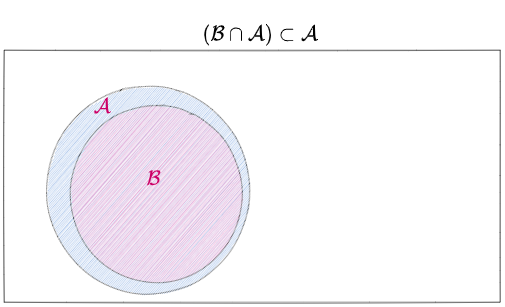
\mathcal{B_0 \subset A}.
P(\mathcal{B_0}) = P(\mathcal{B \cap A}) < P(\mathcal{A}).

\mathcal{B_0 = A}.
P(\mathcal{B_0}) = P(\mathcal{B \cap A}) = P(\mathcal{A}).
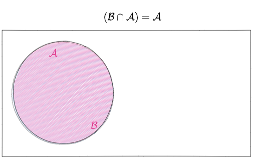
\mathcal{B_0 = A}.
P(\mathcal{B_0}) = P(\mathcal{B \cap A}) = P(\mathcal{A}).
We can see from the above diagrams that,
\mathcal{B_0} \subseteq Aand
P(\mathcal{B_0}) \leq P(\mathcal{A}).Similarly,
P(\mathcal{B_1}) \leq P(\mathcal{A^c}).Hence,
\begin{equation*}
\begin{split}
\mathcal{P_0(B_0)} & \leq \mathcal{P_0(A)} \text{ and} \\
\mathcal{P_1(B_0)} & \leq \mathcal{P_1(A)}. \\
\end{split}
\end{equation*}
Subtracting the second equation from the first,
\mathcal{P_0(B_0) - P_1(B_0) \leq P_0(A) - P_1(A)} \tag{a}.Similarly,
\mathcal{P_0(B_1) - P_1(B_1) \leq P_0(A^c) - P_1(A^c)} \tag{b}.Also,
\begin{equation*}
\begin{split}
\mathcal{P_0(A)} & = \mathcal{\sum_{s \in A} P_0(s)} \text{ and } \\
\mathcal{P_1(A)} & = \mathcal{\sum_{s \in A} P_1(s)}. \\
\end{split}
\end{equation*}
Subtracting the second equation from the first,
\begin{equation*}
\begin{split}
\mathcal{P_0(A) - P_1(A)} & = \mathcal{\sum_{s \in A} P_0(s) - \sum_{s \in A} P_1(s)}  \\
& = \mathcal{\sum_{s \in A} P_0(s) - P_1(s)} \\
& \geq 0. \text{ (since for every } \mathcal{s \in A, P_0(s) \geq P_1(s),} \text{ each term in the sum is non-negative)} \\
\end{split}
\end{equation*}
Since \mathcal{B_0 \subseteq A, s \in B_0 \Rightarrow s \in A}. Hence,
\begin{equation*}
\begin{split}
\mathcal{P_0(B_0) - P_1(B_0)} & = \mathcal{\sum_{s \in B_0} P_0(s) - \sum_{s \in B_0} P_1(s)}  \\
& = \mathcal{\sum_{s \in A} P_0(s) - P_1(s)} \\
& \geq 0. \text{ (since for every } \mathcal{s \in A, P_0(s) \geq P_1(s),} \text{ each term in the sum is non-negative)} \\
\end{split}
\end{equation*}
From equation (a),
\mathcal{\big|P_0(B_0) - P_1(B_0)\big| \leq \big|P_0(A) - P_1(A)\big|} \tag{c}The above equation holds good because taking the absolute value of two non-negative numbers does not change the inequality.
Similarly,
\begin{equation*}
\begin{split}
\mathcal{P_0(A^c) - P_1(A^c)} & = \mathcal{\sum_{s \in A^c} P_0(s) - \sum_{s \in A^c} P_1(s)}  \\
& = \mathcal{\sum_{s \in A^c} P_0(s) - P_1(s)} \\
& \leq 0. \text{ (since for every } \mathcal{s \in A^c, P_0(s) < P_1(s),} \text{ each term in the sum is negative)} \\
\end{split}
\end{equation*}
Substituting the result of the above equation in (b),
\mathcal{P_0(B_1) - P_1(B_1) \leq 0}. \tag{d}\begin{equation*}
\begin{split}
\mathcal{\big|P_0(B) - P_1(B)\big|} & = \mathcal{\big|P_0(B_0 \cup B_1) - P_1(B_0 \cup B_1)\big|} \\
& = \mathcal{\big|P_0(B_0) + P_0(B_1) - P_1(B_0) - P_1(B_1)\big|} \text{ (since } \mathcal{B_0 \text{ and } B_1} \text{ are disjoint sets)} \\
& = \mathcal{\big|P_0(B_0) - P_1(B_0) + P_0(B_1) - P_1(B_1)\big|} \\
& \leq \mathcal{\big|P_0(B_0) - P_1(B_0)\big|} \text{ (from equation (d))} \\
& \leq \mathcal{\big|P_0(A) - P_1(A) \big|}
\end{split}
\end{equation*} Hence we have proved that for any \mathcal{B \subset S \text{ , } \big|P_0(B) - P_1(B)\big| \leq \big|P_0(A) - P_1(A)\big|}.
By definition,
\mathcal{\big\|P_0 - P_1\big\|}_{TV} = \underset{\mathcal{B} \,\subset\, \mathcal{S}}{\text{max}} \mathcal{\big|P_0(B) - P_1(B) \big|}where the maximum is taken over all the subsets \mathcal{B \text{ of } S}.
Since set \mathcal{A} maximizes \mathcal{\big|P_0(B) - P_1(B) \big|},
\mathcal{\big\|P_0 - P_1\big\|}_{TV} = \mathcal{\big|P_0(A) - P_1(A) \big|}.\mathcal{P_0(A) = \sum_{s \in S : P_0(s)\, \geq\, P_1(s)} P_0(s)}\mathcal{P_1(A) = \sum_{s \in S : P_0(s)\, \geq\, P_1(s)} P_1(s)}\begin{equation*}
\begin{split}
\mathcal{\big|P_0(A) - P_1(A) \big|} & = \mathcal{\Big|\sum_{s \in S : P_0(s)\, \geq\, P_1(s)} P_0(s) - \sum_{s \in S : P_0(s)\, \geq\, P_1(s)} P_1(s)\Big|} \\
& = \mathcal{\Big|\sum_{s \in S : P_0(s)\, \geq\, P_1(s)} \big(P_0(s) - P_1(s)\big)\Big|} \\
& = \mathcal{\sum_{s \in S : P_0(s)\, \geq\, P_1(s)}\Big| P_0(s) - P_1(s)\Big|} \\
\end{split}
\end{equation*} The last step follows from the result,
\mathcal{\Bigg|\sum_{i \,=\, 1}^n x_i\Bigg| = \sum_{i \,=\, 1}^n\big|x_i\big| \text{ for all } x_i \in R^+ \text{ (non-negative reals)}}Hence,
\begin{equation*}
\begin{split}
\mathcal{\big\|P_0 - P_1\big\|}_{TV} & = \mathcal{\big|P_0(A) - P_1(A) \big|} \\
& =  \mathcal{\sum_{s \in S : P_0(s)\, \geq\, P_1(s)}\Big| P_0(s) -   P_1(s)\Big|} \tag{2} \\
\end{split}
\end{equation*}
Since \mathcal{A = \{ s \in S : P_0(s) \geq P_1(s)\} \text{ , } A^c = \{ s \in S : P_1(s) > P_0(s)\}}.
For any \mathcal{B \subset S \text{ , } \big|P_1(B) - P_0(B)\big| \leq \big|P_1(A^c) - P_0(A^c)\big|}.
By definition,
\mathcal{\big\|P_1 - P_0\big\|}_{TV} = \underset{\mathcal{B} \,\subset\, \mathcal{S}}{\text{max}} \mathcal{\big|P_1(B) - P_0(B) \big|}.where the maximum is taken over all the subsets \mathcal{B \text{ of } S}.
Since set \mathcal{A^c} maximizes \mathcal{\big|P_1(B) - P_0(B) \big|},
\begin{equation*}
\begin{split}
\mathcal{\big\|P_1 - P_0\big\|}_{TV} & = \mathcal{\big|P_1(A^c) - P_0(A^c) \big|} \\
& = \mathcal{\sum_{s \in S : P_1(s)\, >\, P_0(s)}\Big| P_1(s) -   P_0(s)\Big|} \tag{3} \\
\end{split}
\end{equation*}
Adding equations (2) \text{ and } (3),
\begin{equation*}
\begin{split}
\mathcal{\big\|P_0 - P_1\big\|}_{TV} + \mathcal{\big\|P_1 - P_0\big\|}_{TV} & = \mathcal{\sum_{s \in S : P_0(s)\, \geq\, P_1(s)}\Big| P_0(s) -   P_1(s)\Big|} + \mathcal{\sum_{s \in S : P_1(s)\, >\, P_0(s)}\Big| P_1(s) -   P_0(s)\Big|} \\
& = \mathcal{\sum_{s \in S : P_0(s)\, \geq\, P_1(s)}\Big| P_0(s) -   P_1(s)\Big|} + \mathcal{\sum_{s \in S : P_0(s)\, <\, P_1(s)}\Big| P_0(s) -   P_1(s)\Big|} \\
& = \mathcal{\sum_{s \in S}\Big| P_0(s) -   P_1(s)\Big|} \tag{4} \\
&  \\
& \\
&
\end{split}
\end{equation*}
\mathcal{\big|P_0 - P_1\big|}_{TV} is symmetric since it is a distance function. Therefore,
\mathcal{\big\|P_0 - P_1\big\|}_{TV} = \mathcal{\big\|P_1 - P_0\big\|}_{TV} \tag{5}Using equation (5) \text{ in } (4) we get,
\begin{equation*}
\begin{split}
\mathcal{\big\|P_0 - P_1\big\|}_{TV} + \mathcal{\big\|P_0 - P_1\big\|}_{TV} & = \mathcal{\sum_{s \in S}\Big| P_0(s) -   P_1(s)\Big|} \\
2 \times \mathcal{\big\|P_0 - P_1\big\|}_{TV} & = \mathcal{\sum_{s \in S}\Big| P_0(s) -   P_1(s)\Big|} \\
\mathcal{\big\|P_0 - P_1\big\|}_{TV} & = \frac{1}{2} \mathcal{\sum_{s \in S}\Big| P_0(s) -   P_1(s)\Big|} \\
\end{split}
\end{equation*}
Thus we have proved the equation, \mathcal{\big\|P_0 - P_1\big\|}_{TV} = \frac{1}{2} \sum_{\mathcal{s \in S}} \big|\mathcal{P_0(s) - P_1(s)}\big|.
Also note that, since \mathcal{\big\|P_0 - P_1\big\|}_{TV} = \mathcal{\big\|P_1 - P_0\big\|}_{TV} and,
\begin{equation*}
\begin{split}
\mathcal{\big\|P_0 - P_1\big\|}_{TV} & = \mathcal{\big|P_0(A) - P_1(A) \big|} \text{ and } \\
\mathcal{\big\|P_1 - P_0\big\|}_{TV} & = \mathcal{\big|P_1(A^c) - P_0(A^c) \big|}, \\
\end{split}
\end{equation*}
it follows that,
\mathcal{\big|P_0(A) - P_1(A) \big|} = \mathcal{\big|P_1(A^c) - P_0(A^c) \big|}Hence total variation distance equals either \mathcal{\big|P_0(A) - P_1(A) \big|} \text{ or } \mathcal{\big|P_1(A^c) - P_0(A^c) \big|}.
Now that we have derived some properties of total variation distance, we have to ask ourselves why do we need to measure the distance between two distributions. The larger the distance between two distributions, the easier it is to distinguish them. So the total variation distance, which measures the distance between two distributions, is also a measure of the distinguishability of distributions. We have already discussed at length why distinguishability of distributions matters. Please read this as a refresher before delving into the next section.
Distinguishing Advantage and Distinguishing Distance
We will quickly recapitulate why distinguishability of distributions matters. When an attacker of an encryption scheme gets a distribution of cipher texts, he wants to know whether the distribution is uniform or not. If he gets a uniform distribution, he can do no better than making a random guess about which message was encrypted. On the contrary, if he gets a non-uniform distribution, he can potentially have a better chance than random to attack the encryption scheme. Therefore, he needs to distinguish a uniform distribution from a non-uniform distribution or more generally one distribution from another.
Since an adversary or attacker uses a computer to attack an encryption scheme, it implies that he uses the computer to distinguish distributions. Since the resources (computing power, time etc) of the computer are limited, it suffices to design our encryption schemes such that a computer cannot distinguish a uniform distribution from a non-uniform one, even though mathematically the distributions can be distinguished.
The total variation distance is a mathematical or a theoretical measure of the distance between two distributions. In order for a computer to measure the distance between two distributions accurately (i.e., for the computer’s distance measure to equal the total variation distance) it needs to have unbounded resources i.e., unbounded computing power and time, so that it can observe a very large number of samples of the distribution (say of cipher texts), and can accurately construct the probability distribution (of the cipher texts that it observes).
In cryptography, since we are only concerned with whether our computers can distinguish one distribution from another and since our computers due to their limited resources cannot compute the exact distance between two distributions i.e., the total variation distance, we need to define a new distance function that quantifies the distance between two distributions as measured by a computer. We will call this distance distinguishing distance.
Now that we are convinced that we need a new measure of distance between distributions, how do we go about defining it?
Suppose an adversary (say a computer trying to break an encryption scheme) is given samples from two distributions. It wins if it guesses correctly which distribution that a sample it is given belongs to and loses if it guesses incorrectly. For example, if \mathcal{P_0 \text{ and } P_1} are distributions of cipher texts, the adversary, on getting a cipher text, should be able to guess correctly from which distribution this cipher text is drawn from. The adversary wins if it is able to distinguish the two distributions i.e., if it is able to notice the difference between the distributions. It can notice the difference between the distributions, if the distance between the two distributions is large enough for it to measure this distance. Since the computer operates with limited resources (computing power and time), it has a threshold on the distance between distributions that it can measure. If the distance between two distributions is lesser than this threshold, the distributions will be indistinguishable to the computer. So the adversary’s advantage with respect to the challenger equals the distance between the two distributions as measured by it. Why is this so? Following is an intuitive explanation. We will prove this shortly.
For a deep intuitive understanding of advantage refer to this and this.
As a quick recap,
\begin{equation*}
\begin{split}
\text{Advantage of adversary with respect to challenger} & = \text{Probability that the adversary wins } - \text{Probability that the challenger wins } \\
& =  \text{Probability that the adversary wins } - \text{Probability that the adversary loses } \\
\end{split}
\end{equation*}
The challenger is usually a cryptographic system (like an encryption scheme) and the adversary is an entity trying to break the cryptographic system.
If the distance between two distributions is measurable by the adversary, then it will be able to distinguish one distribution from the other with higher probability, and hence the probability that the adversary wins, namely correctly distinguishes the two distributions, will be higher than the probability it loses i.e., incorrectly distinguishes the two distributions. So it will have a significant advantage, when the distance between the two distributions is measurable.
By the same reasoning, if the distance between two distributions is not measurable by the adversary, its advantage will also be insignificant.
If two distributions are indistinguishable, then the adversary cannot do better than random and hence the probability that it wins will equal the probability that it loses and consequently, its advantage will be zero.
Now that we have an intuitive understanding of why the advantage of the adversary with respect to the challenger is equal to the distance between two distributions as measured by the adversary, we will mathematically prove this equivalence. Since the advantage of the adversary with respect to the challenger is derived from its ability to distinguish the two distributions, we will hence forth refer to it as distinguishing advantage.
Hence,
\text{Advantage of adversary with respect to challenger = Distinguishing Advantage} We will also define distinguishing distance in terms of distinguishing advantage.
The distinguishing advantage is calculated through a game played between the challenger and adversary.
The challenger sends the adversary \mathcal{s \in S} where \mathcal{s} is drawn from either of two distributions \mathcal{P_0 \text{ or } P_1} on the countable set of real numbers \mathcal{S}. The adversary outputs a \mathcal{0 \text{ or } 1} based on its guess of whether \mathcal{s} is drawn from \mathcal{P_0 \text{ or } P_1} respectively. If the adversary guesses correctly it wins the game otherwise it loses. The adversary and challenger might play this game several times.
The game is designed in such a way that the advantage of the adversary is only due to its ability to distinguish one distribution from another and not due to exploiting the challenger’s bias in picking one distribution over another. Suppose the challenger always draws a sample from the distribution \mathcal{P_0}, and the adversary is cognizant of this, then the adversary will have a distinguishing advantage of 1 (the maximum possible advantage) but this advantage is not derived from distinguishing the two distributions but from exploiting the bias of the challenger. Hence to nullify the advantage the adversary might derive from exploiting the challenger’s bias, the challenger will always draw \mathcal{s \in S \text{ from } P_0 \text{ or } P_1} with equal probability i.e.,
\begin{equation*}
\begin{split}
P(\text{Challenger draws } \mathcal{s \in S \text{ from } P_0}) & = \frac{1}{2} \text{ and} \\
P(\text{Challenger draws } \mathcal{s \in S \text{ from } P_1}) & = \frac{1}{2} \\
\end{split}
\end{equation*}
Our game is set up such that the adversary has to guess the correct distribution from two possible distributions so that we can determine the maximum advantage the adversary can have. If it has to guess correctly from three or more distributions, its advantage will be less compared to guessing correctly from two distributions.
Let us assume that the adversary uses a function, \mathcal{D : S \rightarrow \{0, 1\}}, to distinguish the probability distribution \mathcal{P_0 \text{ from } P_1} on the countable set of real numbers \mathcal{S} i.e., \mathcal{D} is a distinguisher function that takes as input a real number \mathcal{s} from the set \mathcal{S} and outputs either a \mathcal{0 \text{ or } 1}.
Mathematically, we can view \mathcal{D} as a special kind of function of a random variable that instead of mapping the set \mathcal{S} of real numbers to another set of real numbers, maps it to either of two values \mathcal{0 \text{ or } 1}. So, \mathcal{D(P_0)} is a random variable that maps the real number \mathcal{s \in S}, where \mathcal{s} is drawn from the probability distribution of \mathcal{P_0}, to either a \mathcal{0 \text{ or } 1}. Similarly \mathcal{D(P_1)}, takes as input \mathcal{s \in S}, where \mathcal{s} is drawn from the probability distribution of \mathcal{P_1} and outputs either a \mathcal{0 \text{ or } 1}.
Hence, P[\mathcal{D(P_0) = 0}] means the probability that \mathcal{D} outputs 0, given \mathcal{s \in S} as input where \mathcal{s} is drawn from the probability distribution of \mathcal{P_0}, i.e.,
P(\mathcal{D} \text{ outputs 0 | } \mathcal{s \in S} \text{ drawn from } \mathcal{P_0} \text{ as input}) = P[\mathcal{D(P_0) = 0}]Similarly,
\begin{equation*}
\begin{split}
P(\mathcal{D} \text{ outputs 1 | } \mathcal{s \in S} \text{ drawn from } \mathcal{P_0} \text{ as input}) & = P[\mathcal{D(P_0) = 1}] \\
P(\mathcal{D} \text{ outputs 0 | } \mathcal{s \in S} \text{ drawn from } \mathcal{P_1} \text{ as input}) & = P[\mathcal{D(P_1) = 0}] \\
P(\mathcal{D} \text{ outputs 1 | } \mathcal{s \in S} \text{ drawn from } \mathcal{P_1} \text{ as input}) & = P[\mathcal{D(P_1) = 1}] \\
\end{split}
\end{equation*}
The probability mass function of the random variable \mathcal{D(P_0)} is defined as the function \mathcal{p_{D(P_0)}} such that,
\begin{equation*}
\begin{split}
\mathcal{p_{D(P_0)}(0)} & = P[\mathcal{D(P_0) = 0}] \text{ and } \\
\mathcal{p_{D(P_0)}(1)} & = P[\mathcal{D(P_0) = 1}]. \\
\end{split}
\end{equation*}
Also by the axioms of probability,
\begin{equation*}
\begin{split}
\mathcal{p_{D(P_0)}(x)} & \geq 0 \text{ , where }
\mathcal{ x \in \{0, 1\}} \text{ and }
 \mathcal{\sum_{x = 0}^1 p_{D(P_0)}(x) = 1}. \tag{6} \\
\end{split}
\end{equation*}
Similarly, the PMF of random variable \mathcal{D(P_1)} is given by,
\begin{equation*}
\begin{split}
\mathcal{p_{D(P_1)}(0)} & = P[\mathcal{D(P_1) = 0}] \text{ and } \\
\mathcal{p_{D(P_1)}(1)} & = P[\mathcal{D(P_1) = 1}]. \\
\end{split}
\end{equation*}
And by the axioms of probability,
\begin{equation*}
\begin{split}
\mathcal{p_{D(P_1)}(x)} & \geq 0 \text{ , where } \mathcal{ x \in \{0, 1\}} \text{ and } \mathcal{\sum_{x = 0}^1 p_{D(P_1)}(x) = 1}. \tag{7} \\
\end{split}
\end{equation*}
Since to calculate the distinguishing advantage, we need to know the probability that the adversary wins and its complement i.e., the probability that it loses, the next question to ask is, how does the adversary win?
The adversary wins in two ways:
- The adversary is given an input \mathcal{s \in S} that is drawn from the distribution of \mathcal{P_0} and it outputs \mathcal{0}.
- The adversary is given an input \mathcal{s \in S} that is drawn from the distribution of \mathcal{P_1} and it outputs \mathcal{1}.
\begin{equation*}
\begin{split}
P(\text{Adversary wins}) & = P(\text{Challenger draws } \mathcal{s \in S \text{ from } P_0}) \times  P(\mathcal{D} \text{ outputs 0 | } \mathcal{s \in S} \text{ drawn from } \mathcal{P_0} \text{ as input}) \\
& \;\;\;+ P(\text{Challenger draws } \mathcal{s \in S \text{ from } P_1}) \times  P(\mathcal{D} \text{ outputs 1 | } \mathcal{s \in S} \text{ drawn from } \mathcal{P_1} \text{ as input})\\
& = \frac{1}{2} \times P[\mathcal{D(P_0) = 0}] + \frac{1}{2} \times P[\mathcal{D(P_1) = 1}] \\
\end{split}
\end{equation*}
Similarly, the adversary loses in two ways:
- The adversary is given an input \mathcal{s \in S} that is drawn from the distribution of \mathcal{P_0} and it outputs \mathcal{1}.
- The adversary is given an input \mathcal{s \in S} that is drawn from the distribution of \mathcal{P_1} and it outputs \mathcal{0}.
P(\text{Adversary loses}) = \frac{1}{2} \times P[\mathcal{D(P_0) = 1}] + \frac{1}{2} \times P[\mathcal{D(P_1) = 0}]From equations \mathcal{(6) \text{ and } (7)},
\begin{equation*}
\begin{split}
P[\mathcal{D(P_0) = 0}] + P[\mathcal{D(P_0) = 1}] &= 1 \text{ and} \\
P[\mathcal{D(P_1) = 0}] + P[\mathcal{D(P_1) = 1}] &= 1. \\
\end{split}
\end{equation*}
Hence,
\begin{equation*}
\begin{split}
P[\mathcal{D(P_0) = 0}] &= 1 - P[\mathcal{D(P_0) = 1}]  \text{ and}  \tag{8} \\
P[\mathcal{D(P_1) = 0}] &= 1 - P[\mathcal{D(P_1) = 1}].\\
\end{split}
\end{equation*}
\begin{align*}
\textit{Distinguishing Advantage} & = \big|\text{Advantage of adversary with respect to challenger}\big| \\
& = \big|P(\text{Adversary wins}) - P(\text{Challenger wins})\big| \\
& = \big|P(\text{Adversary wins}) - P(\text{Adversary loses})\big| \\
& = \frac{1}{2} \times \Big\{\big|P[\mathcal{D(P_0) = 0}] + P[\mathcal{D(P_1) = 1}] - P[\mathcal{D(P_0) = 1}] - P[\mathcal{D(P_1) = 0}]\big|\Big\} \\
& = \frac{1}{2} \times \Big\{\big|P[\mathcal{D(P_0) = 0}] - P[\mathcal{D(P_1) = 0}] + P[\mathcal{D(P_1) = 1}] - P[\mathcal{D(P_0) = 1}]\big|\Big\} \\
& = \frac{1}{2} \times \Big\{\big|1 - P[\mathcal{D(P_0) = 1}] - 1 + P[\mathcal{D(P_1) = 1}] + P[\mathcal{D(P_1) = 1}] - P[\mathcal{D(P_0) = 1}]\big|\Big\} \\
&\hspace{0.5 cm} \text{(substituting equation (8) in the above equation)}\\
& = \frac{1}{2} \times \Big\{2 \times \big|P[\mathcal{D(P_1) = 1}] - P[\mathcal{D(P_0) = 1}]\big|\Big\} \\
& = \big|P[\mathcal{D(P_1) = 1}] - P[\mathcal{D(P_0) = 1}]\big| \\
& = \big|P[\mathcal{D(P_0) = 1}] - P[\mathcal{D(P_1) = 1}]\big| &\text{(9)}
\end{align*} The above equation forms the basis for our security proofs in cryptography. To prove that a cryptographic system is secure, we use the distinguishing advantage to calculate an adversary’s advantage with respect to the cryptographic system. If the adversary’s advantage is below a certain threshold (we call this advantage negligible; we will discuss what negligible means in later) then we deem the cryptographic system to be secure. Since distinguishing advantage is the tenet in proving the security of cryptographic systems it makes sense to develop an intuitive understanding of it.
The table below enumerates the various inputs to the distinguisher, its outputs as well as the probabilities of a particular input resulting in a particular output.

Since P[\mathcal{D(P_0) = 0}] \text{ and } P[\mathcal{D(P_0) = 1}] are probabilities of two complementary events (the probabilities sum to 1), we can view them as conveying the same information. For the same reason, P[\mathcal{D(P_1) = 0}] \text{ and } P[\mathcal{D(P_1) = 1}] also conveys the same information. Hence in the equation of the distinguishing advantage, we two out of the four terms are redundant since they convey the same information. This is shown below.

Hence we can remove the redundant terms (shown in light blue and light red) and get the following equation for distinguishing advantage.

which is equivalent to,

It should be noted that we can remove any of the two redundant terms i.e., keep the probabilities shown in the light blue and light pink and remove their complements shown respectively in darker blue and darker pink. Thus,

Why is Distinguishing Advantage an absolute value?
The adversary wins if it correctly guesses which of the two distributions it is given a sample from and loses otherwise. So if it guesses correctly a lot more times than it guesses wrongly, then it is able to distinguish the two distributions \mathcal{P_0} and \mathcal{P_1}. But wait. Why does the definition of distinguishing advantage have an absolute sign? This seems to say that even when the adversary guesses wrongly a lot more times than it guesses rightly it still has an advantage. Why is this so? This is because even if it guesses wrongly, when it plays this game several times it will realize that it is losing many more times than it is winning and hence it will inverse its strategy and guess correctly i.e., where initially it output \mathcal{0}, it will now output \mathcal{1} and hence guess correctly. Even if it was initially making the wrong guess, it was still able to distinguish the two distributions and hence it has an advantage.
For an intuitive understanding of why distinguishing advantage is an absolute value refer here.
Hence if distributions \mathcal{P_0 \text{ and } P_1} are distinguishable by the adversary, then the probability that \mathcal{D} outputs \mathcal{1} on getting \mathcal{s \in S} drawn from \mathcal{P_0} as its input will be significantly different than the probability that \mathcal{D} outputs \mathcal{1} on getting \mathcal{s \in S} drawn from \mathcal{P_1} as its input. Hence to calculate the distinguishing advantage we only need the absolute difference between P[\mathcal{D(P_0) = 1}] \text{ and } P[\mathcal{D(P_1) = 1}] since we only care about the magnitude of their difference.
What is the range of values distinguishing advantage can take?
What is the minimum value of \big|P[\mathcal{D(P_0) = 1}] - P[\mathcal{D(P_1) = 1}]\big|?
Since \big|P[\mathcal{D(P_0) = 1}] - P[\mathcal{D(P_1) = 1}]\big| is positive, its minimum value occurs when P[\mathcal{D(P_0) = 1}] = P[\mathcal{D(P_1) = 1}], in which case it is 0.
What is the maximum value of \big|P[\mathcal{D(P_0) = 1}] - P[\mathcal{D(P_1) = 1}]\big|?
Since P[\mathcal{D(P_0) = 1}] and P[\mathcal{D(P_1) = 1}] are probabilities, the minimum value they can take is 0 and the maximum value is 1. So \big|P[\mathcal{D(P_0) = 1}] - P[\mathcal{D(P_1) = 1}]\big| is maximized when one of them takes the value 0 and the other takes the value 1. Hence the maximum value of \big|P[\mathcal{D(P_0) = 1}] - P[\mathcal{D(P_1) = 1}]\big| is 1.
Hence distinguishing advantage will include all real numbers between 0 and 1 (including 0 and 1) i.e., \big[0, 1\big].
Alternate notation for deriving Distinguishing Advantage
Sometimes an alternate notation is used in deriving distinguishing advantage. We will briefly describe this notation and derive distinguishing advantage in terms of it.
Let \mathcal{W_0} be the event that the adversary (or equivalently the distinguisher \mathcal{D}) outputs \mathcal{1} when given as input \mathcal{s \in S} drawn from distribution \mathcal{P_0}. Hence,
P[\mathcal{W_0}] = P[\mathcal{D} \text{ outputs 1 | } \mathcal{s \in S} \text{ drawn from } \mathcal{P_0} \text{ as input}]. So,
P[\mathcal{W_0}] = P[\mathcal{D(P_0) = 1}]Similarly, let
\begin{equation*}
\begin{split}
P[\mathcal{W_0'}] & = P[\mathcal{D(P_0) = 0}], \\
P[\mathcal{W_1}] & = P[\mathcal{D(P_1) = 1}] \text{ and} \\
P[\mathcal{W_1'}] & = P[\mathcal{D(P_1) = 0}]
\end{split}
\end{equation*}
By the axiom of probability,
\begin{equation*}
\begin{split}
P[\mathcal{W_0}] + P[\mathcal{W_0'}] & = 1 \text{ and} \\
P[\mathcal{W_1}] + P[\mathcal{W_1'}] & = 1 \\ \tag{8a}
\end{split}
\end{equation*}
\begin{equation*}
\begin{split}
\textit{Distinguishing Advantage} & = \big|\text{Advantage of adversary with respect to challenger}\big| \\
& = \big|P(\text{Adversary wins}) - P(\text{Challenger wins})\big| \\
& = \big|P(\text{Adversary wins}) - P(\text{Adversary loses})\big| \\
& = \frac{1}{2} \times \Big\{\big|P[\mathcal{W_0'}] + P[\mathcal{W_1}] - P[\mathcal{W_0}] - P[\mathcal{W_1'}]\big|\Big\} \\
& = \frac{1}{2} \times \Big\{\big|P[\mathcal{W_0'}] - P[\mathcal{W_1'}] + P[\mathcal{W_1}] - P[\mathcal{W_0}]\big|\Big\} \\
& = \frac{1}{2} \times \Big\{\big|1 - P[\mathcal{W_0}] - 1 + P[\mathcal{W_1}] + P[\mathcal{W_1}] - P[\mathcal{W_0}]\big|\Big\} \\
&\hspace{0.5 cm} \text{(substituting equation (8a) in the above equation)}\\
& = \frac{1}{2} \times \Big\{2 \times \big|P[\mathcal{W_1}] - P[\mathcal{W_0}]\big|\Big\} \\
& = \big|P[\mathcal{W_1}] - P[\mathcal{W_0}] \big| \\
& = \big|P[\mathcal{W_0}] - P[\mathcal{W_1}] \big| \\
\end{split}
\end{equation*} From equation \mathcal{(9)},
\big|P[\mathcal{D(P_0) = 1}] - P[\mathcal{D(P_1) = 1}]\big| = \big|P[\mathcal{W_0}] - P[\mathcal{W_1}] \big|For a given challenger \mathcal{C} and a given adversary \mathcal{A}, the advantage of adversary \mathcal{A} with respect to challenger \mathcal{C} is denoted by \text{Adv}\mathcal{[A, C]} and is defined as,
\text{Adv}\mathcal{[A, C]} = \big|P[\mathcal{W_0}] - P[\mathcal{W_1}] \big|where \mathcal{W_0} is the event that the adversary \mathcal{A} outputs \mathcal{1} when given as input \mathcal{s \in S} (where \mathcal{S} is a countable set of real numbers) drawn from distribution \mathcal{P_0} and \mathcal{W_1} is the event that the adversary \mathcal{A} outputs \mathcal{1} when given as input \mathcal{s \in S} drawn from distribution \mathcal{P_1}.
The following is a graphical explanation of the above equation.

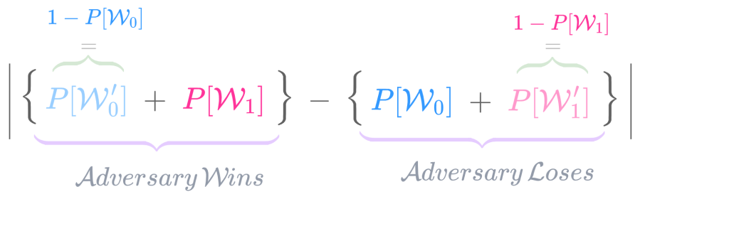
As already explained above, removing the redundant terms we get,

which is equivalent to,
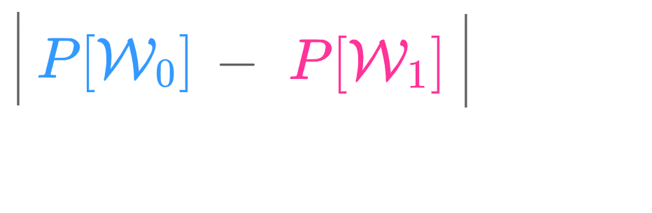
As already discussed, we can remove any of the two redundant terms i.e., keep the probabilities shown in the light blue and light pink and remove their complements shown respectively in darker blue and darker pink. Thus,

Bias
For an intuitive understanding of bias please refer here and here.
Suppose an adversary is given a sample drawn from one of two distributions and it has to guess which distribution the sample is drawn from. If an adversary’s only chance of winning is by making a random guess, then its probability of winning is \mathcal{\frac{1}{2}}, which is also its probability of losing. Suppose on the contrary, on getting the sample it is able to guess correctly which distribution the sample is drawn from with a probability greater than \mathcal{\frac{1}{2}}. Bias measures this deviation from the random guess i.e., from a uniform distribution. If the adversary guesses correctly with probability \mathcal{\frac{1}{2} + \epsilon^\prime}, then \mathcal{\epsilon^\prime} is the bias.
Bias is defined as the measure of the absolute difference between probabilities of an event occurring in a given distribution and the same event occurring in a uniform distribution.
Suppose the probability that the adversary wins is \mathcal{\frac{1}{2} + \epsilon^\prime}. Then the probability that it loses is \mathcal{1 - (\frac{1}{2} + \epsilon^\prime) = \frac{1}{2} - \epsilon^\prime}.
\begin{equation*}
\begin{split}
\textit{Distinguishing Advantage, } \epsilon & = \big|\text{Advantage of adversary with respect to challenger}\big| \\
& = \big|P(\text{Adversary wins}) - P(\text{Adversary loses})\big| \\
& = \Bigg|\bigg(\mathcal{\frac{1}{2} + \epsilon^\prime}\bigg) - \bigg(\mathcal{\frac{1}{2} - \epsilon^\prime}\bigg) \Bigg| \\
& = 2 \times \epsilon^\prime \\
& = 2 \times \textit{Bias}
\end{split}
\end{equation*}
Hence,
\textit{Bias} = \frac{1}{2} \times \textit{Distinguishing Advantage}If the probability that the adversary wins is \mathcal{\frac{1}{2} - \epsilon^\prime}, then,
\begin{equation*}
\begin{split}
\textit{Distinguishing Advantage, } \epsilon & = \big|\text{Advantage of adversary with respect to challenger}\big| \\
& = \big|P(\text{Adversary wins}) - P(\text{Adversary loses})\big| \\
& = \Bigg|\bigg(\mathcal{\frac{1}{2} - \epsilon^\prime}\bigg) - \bigg(\mathcal{\frac{1}{2} + \epsilon^\prime}\bigg) \Bigg| \\
& = \big|-2\times \epsilon^\prime\big|\\
& = 2 \times \epsilon^\prime \\
& = 2 \times \textit{Bias}
\end{split}
\end{equation*}
Definition of Distinguishing Advantage
We will define distinguishing advantage of \mathcal{D}, as follows:
A distinguisher is a function \mathcal{D : S \rightarrow \{0, 1\}}, where \mathcal{S} is a countable set of real numbers. If \mathcal{P_0 \text{ and } P_1} are probability distributions on \mathcal{S}, the advantage of \mathcal{D} in distinguishing \mathcal{P_0 \text{ from } P_1} is called distinguishing advantage of \mathcal{D}. It is denoted by \text{Adv}_D(\mathcal{P_0, P_1}) and is defined as,
\text{Adv}_D(\mathcal{P_0, P_1}) = \big|P[\mathcal{D(P_0) = 1}] - P[\mathcal{D(P_1) = 1}]\big|. \tag{10}The distinguishing advantage of \mathcal{D} is also denoted by \mathcal{\epsilon}.
We will now prove that the distinguishing advantage of \mathcal{D}, \mathcal{\epsilon}, is equal to the total variation distance between the distributions \mathcal{p_{D(P_0)} \text{ and } p_{D(P_1)}}.
In order to calculate the total variation distance between the distributions \mathcal{p_{D(P_0)} \text{ and } p_{D(P_1)}}, we will first calculate the \mathcal{L_1} distance between \mathcal{p_{D(P_0)} \text{ and } p_{D(P_1)}} and then calculate total variation distance by using its relationship to \mathcal{L_1} distance (we have already proved that total variation distance is half the \mathcal{L_1} distance).
The \mathcal{L_1} distance between the probability distributions \mathcal{p_{D(P_0)} \text{ and } p_{D(P_1)}} is given by,
\begin{equation*}
\begin{split}
\mathcal{\big\|p_{D(P_0)} - p_{D(P_1)}\big\|}_1 & = \mathcal{ \sum_{x \,\in\, \{0, 1\}} \big|p_{D(P_0)}(x) - p_{D(P_1)} (x)\big|} \\
& = \mathcal{\big|p_{D(P_0)}(0) - p_{D(P_1)} (0)\big| + \big|p_{D(P_0)}(1) - p_{D(P_1)} (1)\big|} \\
& = \big|P[\mathcal{D(P_0) = 0}] - P[\mathcal{D(P_1) = 0}]\big| + \big|P[\mathcal{D(P_0) = 1}] - P[\mathcal{D(P_1) = 1}]\big| \\
& = \big|1 - P[\mathcal{D(P_0) = 1}] - 1 + P[\mathcal{D(P_1) = 1}]\big| + \big|P[\mathcal{D(P_0) = 1}] - P[\mathcal{D(P_1) = 1}]\big| \\
&\hspace{0.5 cm} \text{(substituting equation (8) in the above equation)}\\
& = \big|- P[\mathcal{D(P_0) = 1}] + P[\mathcal{D(P_1) = 1}]\big| + \big|P[\mathcal{D(P_0) = 1}] - P[\mathcal{D(P_1) = 1}]\big| \\
& = \big|P[\mathcal{D(P_0) = 1}] - P[\mathcal{D(P_1) = 1}]\big| + \big|P[\mathcal{D(P_0) = 1}] - P[\mathcal{D(P_1) = 1}]\big| \\
&\hspace{0.5 cm} \text{(since } \mathcal{\big|a -b\big| = \big|b -a\big|} \text{ for all \{a, b\}} \mathcal{\in R}) \\
& = \mathcal{2 \times \big|P[\mathcal{D(P_0) = 1}] - P[\mathcal{D(P_1) = 1}]\big|} \\
& = 2 \times \text{Adv}_D(\mathcal{P_0, P_1})\\
&\hspace{0.5 cm} \text{(from equation (10))}\\
\end{split}
\end{equation*}
We have already proved that,
\begin{equation*}
\begin{split}
\mathcal{\big\|P_0 - P_1\big\|}_{TV} & = \frac{1}{2} \mathcal{\big\|P_0 - P_1\big\|}_1 \\
\end{split}
\end{equation*}
See equation \mathcal{(1)} onwards for proof.
Therefore,
\begin{equation*}
\begin{split}
\mathcal{\big\|p_{D(P_0)} - p_{D(P_1)}\big\|}_{TV} & = \mathcal{\frac{1}{2} \big\|p_{D(P_0)} - p_{D(P_1)}\big\|}_1 \\
& = \mathcal{\frac{1}{2} \times 2 \times \big|P[\mathcal{D(P_0) = 1}] - P[\mathcal{D(P_1) = 1}]\big|} \\
& = \mathcal{\big|P[\mathcal{D(P_0) = 1}] - P[\mathcal{D(P_1) = 1}]\big|} \tag{11}\\\\\\
\end{split}
\end{equation*}
From equations \mathcal{(10) \text{ and } (11)},
\text{Adv}_{D}(\mathcal{P_0, P_1}) = \mathcal{\big\|p_{D(P_0)} - p_{D(P_1)}\big\|}_{TV} \tag{12}i.e., distinguishing advantage of \mathcal{D} equals the total variation distance between the distributions \mathcal{p_{D(P_0)} \text{ and } p_{D(P_1)}}.
\mathcal{\big\|p_{D(P_0)} - p_{D(P_1)}\big\|}_{TV} is the total variation distance between distributions \mathcal{p_{D(P_0)} \text{ and } p_{D(P_1)}} and also the distinguishing distance between distributions \mathcal{P_0 \text{ and } P_1} with respect to the distinguisher \mathcal{D}.
Definition of Distinguishing Distance
We define the distinguishing distance as follows:
A distinguisher is a function \mathcal{D : S \rightarrow \{0, 1\}} where \mathcal{S} is a countable set of real numbers. If \mathcal{P_0 \text{ and } P_1} are probability distributions on \mathcal{S}, the distinguishing distance between \mathcal{P_0 \text{ and } P_1} is denoted by \mathcal{\big\|P_0 - P_1\big\|}_D and is defined as,
\mathcal{\big\|P_0 - P_1\big\|}_D = \mathcal{\big|P[\mathcal{D(P_0) = 1}] - P[\mathcal{D(P_1) = 1}]\big|}From equation \mathcal{(11) \text{ and } (12)} it follows that,
\begin{equation*}
\begin{split}
\text{Adv}_{D}(\mathcal{P_0, P_1}) & = \mathcal{\big\|p_{D(P_0)} - p_{D(P_1)}\big\|}_{TV} \\
&= \mathcal{\big|P[\mathcal{D(P_0) = 1}] - P[\mathcal{D(P_1) = 1}]\big|}\\
& = \mathcal{\big\|P_0 - P_1\big\|}_D \\
& = 2 \times \textit{Bias}
\end{split}
\end{equation*}
The above equation implies that the distinguishing advantage of \mathcal{D} in distinguishing the two distributions \mathcal{P_0 \text{ and } P_1} is equal to the distinguishing distance between the distributions \mathcal{P_0 \text{ and } P_1} which is also equal to the total variation distance between the distributions \mathcal{p_{D(P_0)} \text{ and } p_{D(P_1)}}.
Since the computer operates with limited resources (computing power and time), it has a threshold on the distance between distributions that it can measure. If the distance between two distributions is lower than this threshold, the distributions will be indistinguishable to the computer. It cannot measure this distance because in order to measure the distance between two distributions accurately, the computer would need to draw a very large number of samples from the two distributions to be able to construct their probability distributions accurately which would in turn require more time and computing power which is unavailable to it. Also the algorithm that the computer uses to distinguish the two distributions might not be accurate in distinguishing them and the computer might not have the resources to find the best algorithm that distinguishes the two distributions accurately. For a mathematical proof of why the algorithm matters refer to this.
So the distinguishing distance i.e., the distance between two distributions as measured by a computer using a distinguisher function will always be less than the total variational distance, the mathematical measure of distance between two distributions. The distinguishing distance can equal the total variational distance only if an adversary has unbounded resources.
Now let us translate the above discussion into an equation and prove the validity of the equation.
For any distinguisher \mathcal{D},
\mathcal{\big\|P_0 - P_1\big\|}_D \leq \mathcal{\big\|P_0 - P_1\big\|}_{TV}.\mathcal{\big\|P_0 - P_1\big\|}_D = \mathcal{\big\|P_0 - P_1\big\|}_{TV} if an adversary using a distinguisher \mathcal{D} to distinguish the two distributions has unbounded resources (computing power and time).
We have already proved that \text{Adv}_{D}(\mathcal{P_0, P_1}) = \mathcal{\big\|P_0 - P_1\big\|}_D. Hence, \text{Adv}_{D}(\mathcal{P_0, P_1}) \leq \mathcal{\big\|P_0 - P_1\big\|}_{TV}.
In practice, the distinguisher function \mathcal{D(\cdot)} is a probabilistic algorithm and so it introduces a degree of randomness in its logic. It does so by randomly picking a string \mathcal{r} from a uniform distribution on some set \mathcal{R} as an auxiliary input to guide its behavior. This uniform distribution on set \mathcal{R} is independent of the distributions \mathcal{P_0 \text{ and } P_1}.
Hence \mathcal{D(\cdot)} takes two inputs, namely, \mathcal{r \in R \text{ and } s \in S} and outputs either a \mathcal{0 \text{ or } 1}.
Let \mathcal{S_{r_0} = \{s \in S : D(r_0, s) = 1\}}. Therefore,
\begin{equation*}
\begin{split}
\mathcal{\big\|P_0 - P_1\big\|_D} & = \big|P[\mathcal{D(r, P_0) = 1}] - P[\mathcal{D(r, P_1) = 1}]\big| \\
& = \mathcal{\Big|\sum_{r_0 \in R}} P(r = r_0) \big\{ P\big[\mathcal{D(r_0, P_0) = 1 \big| r = r_0}\big] - P\big[\mathcal{D(r_0, P_1) = 1 \big| r = r_0}\big]\big\} \Big| \\
& = \mathcal{\Big|\sum_{r_0 \in R}} P(r = r_0) \big\{ P\big[\mathcal{D(r_0, P_0) = 1}\big] - P\big[\mathcal{D(r_0, P_1) = 1}\big]\big\} \Big| \text{ (since }  \mathcal{r \text{ is independent of distributions } P_0 \text{ and } P_1)}\\
& = \mathcal{\Big|\sum_{r_0 \in R}} P(r = r_0) \mathcal{\big[ P_0(S_{r_0}) - P_1(S_{r_0})\big] \Big|} \\
& \leq \mathcal{\sum_{r_0 \in R}} P(r = r_0) \mathcal{\Big|\big[ P_0(S_{r_0}) - P_1(S_{r_0})\big] \Big|} \\
& \leq \mathcal{\sum_{r_0 \in R}} P(r = r_0) \mathcal{\Big|\big[ P_0(A) - P_1(A)\big] \Big|} \\
\end{split}
\end{equation*}
We have already proved that for any \mathcal{B \subset S \text{ , } \big|P_0(B) - P_1(B)\big| \leq \big|P_0(A) - P_1(A)\big|}. Refer this for proof.
Hence,
\begin{equation*}
\begin{split}
\mathcal{\big\|P_0 - P_1\big\|_D} & \leq \mathcal{\sum_{r_0 \in R}} P(r = r_0) \mathcal{\Big|\big[ P_0(A) - P_1(A)\big] \Big|} \\
& \leq \mathcal{\frac{1}{|R|} \sum_{r_0 \in R}} \mathcal{\Big|\big[ P_0(A) - P_1(A)\big] \Big|}  \\
& \leq \mathcal{\Big|\big[ P_0(A) - P_1(A)\big] \Big|} \\
& \leq \mathcal{\big\|P_0 - P_1\big\|}_{TV}
\end{split}
\end{equation*}
Hence we have proved that for any distinguisher \mathcal{D},
\mathcal{\big\|P_0 - P_1\big\|}_D \leq \mathcal{\big\|P_0 - P_1\big\|}_{TV}For any distinguisher \mathcal{D \text{ and } r \in R}, we can define a set \mathcal{S_r} such that \mathcal{S_r = \{s \in S : D(r, s) = 1\}}. We have already proved that
\mathcal{\big\|P_0 - P_1\big\|}_{TV} = \mathcal{\big|P_0(A) - P_1(A) \big|} where \mathcal{A = \{s \in S : P_0(s) \geq P_1(s)\}}.
Suppose an adversary has unbounded resources (i.e., computing power and time), it could then iterate through all possible distinguishers and all possible \mathcal{r \in R} to find the distinguisher \mathcal{D_0 \text{ and } r_0 \in R} such that \mathcal{S_{r_0} = A}, where \mathcal{S_{r_0} = \{s \in S : D_0(r_0, s) = 1\}}. Therefore,
\begin{equation*}
\begin{split}
\mathcal{\big\|P_0 - P_1\big\|_D} & = \big|P[\mathcal{D(r, P_0) = 1}] - P[\mathcal{D(r, P_1) = 1}]\big| \\
& = \Big|P(r = r_0) \big\{ P\big[\mathcal{D(r_0, P_0) = 1 \big| r = r_0}\big] - P\big[\mathcal{D(r_0, P_1) = 1 \big| r = r_0}\big]\big\} \Big| \\
& = \Big| P(r = r_0) \big\{ P\big[\mathcal{D(r_0, P_0) = 1}\big] - P\big[\mathcal{D(r_0, P_1) = 1}\big]\big\} \Big| \text{ (since }  \mathcal{r \text{ is independent of distributions } P_0 \text{ and } P_1)}\\
& = \Big| P\big[\mathcal{D(r_0, P_0) = 1}\big] - P\big[\mathcal{D(r_0, P_1) = 1}\big] \Big| \text{ (since } \mathcal{D_0} \text{ chooses } \mathcal{r_0} \text{ with probability 1, } P(\mathcal{r = r_0) = 1}) \\
& = \Big| \mathcal{P_0(S_{r_0}) - P_1(S_{r_0})} \Big| \text{ (since } \mathcal{S_{r_0} = \{s \in S : D_0(r_0, s) = 1\}}) \\
& = \Big| \mathcal{P_0(A) - P_1(A)} \Big| \text{ (since } \mathcal{S_{r_0} = A}) \\
& = \mathcal{\big\|P_0 - P_1\big\|}_{TV} \\
\end{split}
\end{equation*}
Since \mathcal{D_0} uses only one particular value \mathcal{r_0} from the set \mathcal{R}, when an adversary has unbounded resources, \mathcal{D_0} is no longer a probabilistic algorithm but becomes a deterministic algorithm. This is because since the adversary has unbounded resources, it can iterate through all possible \mathcal{r \in R} and choose the \mathcal{r} that maximizes \big|P[\mathcal{D_0(r, P_0) = 1}] - P[\mathcal{D_0(r, P_1) = 1}]\big|. When the resources of an adversary is bounded, it might not be able to exhaust all possible \mathcal{r \in R} and hence we take the average of all possible distances computed by it.
Four Equivalent Definitions of Total Variation Distance Between Two Distributions
To summarize, if \mathcal{P_0 \text{ and } P_1} are two probability distributions on a countable set of real numbers \mathcal{S}, then the total variation distance between them is defined in four equivalent ways as follows:
- \mathcal{\big\|P_0 - P_1\big\|}_{TV} = \underset{\mathcal{B} \,\subset\, \mathcal{S}}{\text{max}} \mathcal{\big|P_0(B) - P_1(B) \big|}.
- \mathcal{\big\|P_0 - P_1\big\|}_{TV} = \frac{1}{2} \mathcal{\big\|P_0 - P_1\big\|}_1 = \frac{1}{2}\underset{\mathcal{s \in S}}{\sum} \mathcal{\big|P_0(s) - P_1(s) \big|}.
- \mathcal{\big\|P_0 - P_1\big\|}_{TV} = \underset{\mathcal{D : S \rightarrow \{0, 1\}}}{\text{max}} \mathcal{\big|P[\mathcal{D(P_0) = 1}] - P[\mathcal{D(P_1) = 1}]\big|},
where \mathcal{D(\cdot)} is a distinguisher function that distinguishes \mathcal{P_0 \text{ from } P_1}. \mathcal{D}(P_0) means \mathcal{D} takes as input \mathcal{s \in S}, where \mathcal{s} is drawn from the distribution \mathcal{P_0} and outputs either 0 or 1. Similarly for \mathcal{D}(P_1). - \mathcal{\big\|P_0 - P_1\big\|}_{TV} = \underset{\mathcal{A : S \rightarrow \{0, 1\}}}{\text{max}} \mathcal{\big|P[\mathcal{W_0}] - P[\mathcal{W_1}]\big|},
where \mathcal{W_0} is the event that the adversary \mathcal{A} outputs \mathcal{1} when given as input \mathcal{s \in S} drawn from \mathcal{P_0} and \mathcal{W_1} is the event that the adversary \mathcal{A} outputs \mathcal{1} when given as input \mathcal{s \in S} drawn from \mathcal{P_1}.
Total Variation Distance Between Two Random Variables
The total variation distance between two random variables is the total variation distance between their corresponding distributions.
Four Equivalent Definitions of Total Variation Distance Between Two Random Variables
If X \text{ and } Y are two random variables taking values from a countable set of real numbers \mathcal{R}, then the total variation distance between them is defined in four equivalent ways as follows:
- \big\|X - Y\big\|_{TV} = \underset{\mathcal{R'} \,\subset\, \mathcal{R}}{\text{max}} \big|P(X \in \mathcal{R'}) - P(Y \in \mathcal{R'}) \big|.
- \big\|X - Y\big\|_{TV} = \frac{1}{2} \Big\|X - Y\Big\|_1 = \frac{1}{2}\underset{\mathcal{r \in R}}{\sum} \big|P(X = r) - P(Y = r) \big|.
- \big\|X - Y\big\|_{TV} = \underset{\mathcal{D : R \rightarrow \{0, 1\}}}{\text{max}} \big|P[\mathcal{D}(X) = 1] - P[\mathcal{D}(Y) = 1]\big|,
where \mathcal{D(\cdot)} is a distinguisher function that distinguishes the probability distributions of X \text{ and } Y. \mathcal{D}(X) means \mathcal{D} takes as input \mathcal{r \in R}, where \mathcal{r} is drawn from the distribution of X and outputs either 0 or 1. Similarly for \mathcal{D}(Y). - \big\|X - Y\big\|_{TV} = \underset{\mathcal{A : R \rightarrow \{0, 1\}}}{\text{max}} \mathcal{\big|P[\mathcal{W_0}] - P[\mathcal{W_1}]\big|},
where \mathcal{W_0} is the event that the adversary \mathcal{A} outputs \mathcal{1} when given as input \mathcal{r \in R} drawn from the distribution of X and \mathcal{W_1} is the event that the adversary \mathcal{A} outputs \mathcal{1} when given as input \mathcal{r \in R} drawn from the distribution of Y.
We can prove the equivalence of the above definitions for random variables similar to the proof we have done for distributions.
Before we proceed further, we will take a little detour and refresh our knowledge on preimages.
Preimage
The word “preimage” is used in two related ways as discussed below.
Preimage of an element of a set
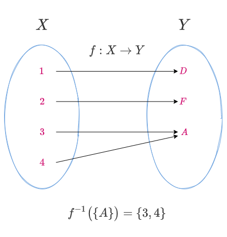
If f : X \rightarrow Y is any function, then the preimage (or inverse image) of an element y \in Y under f, denoted by f^{-1}\big(\{y\}\big), is the set of all elements of X that are related to y under f. That is,
f^{-1} \big(\{y\}\big) = \{x \in X : f(x) = y\}\text{The following diagram is a pictorial representation of the function } f : \{ 1, 2, 3, 4 \} \to \{ D, F, A \} \text{ defined by }\left\{\begin{matrix}
1 \mapsto D, \\
2 \mapsto F, \\
3 \mapsto A, \\
4 \mapsto A.
\end{matrix}\right. and the preimage of f^{-1}\big({y}\big) \text{ where } y \in Y \text{ and } y = A.
Preimage of a subset
Similarly, if S is a subset of Y\!\!, then the preimage of S under f, denoted by f^{-1}(S), is the set of all elements of X that are related to elements in S under f.
That is,
f^{-1}(S) = \{x \in X : f(x) \in S\}The following diagram is a pictorial representation of the function f defined as above and f^{-1}(S) \text{ where } S \subset Y.

As another example, let us consider the function f : \{-1, 1, -2, 2, -3, 3\} \rightarrow \{1, 4, 9\} \text{ defined by } f(x) = x^2. The preimage of the set \{4, 9\} under f is \{-2, 2, -3, 3\} and is pictorially shown below.

Total Variation Distance between functions of two random variables
If \mathcal{S \text{ and } T} are countable sets of real numbers and X \text{ and } Y are random variables with support \mathcal{S}, then for any function, \mathcal{f : S \rightarrow T} ,\big\|f(X) - f(Y)\big\|_{TV} \leq \big\|X - Y\big\|_{TV}.
\begin{equation*}
\begin{split}
\big\|f(X) - f(Y)\big\|_{TV}  & = \big|P[f(X) \in \mathcal{T'}] - P[f(Y) \in \mathcal{T'}]\big| \text{ (for some } \mathcal{T' \subset T)} \\
& = \big|P[X \in f^{-1}(\mathcal{T'})] - P[Y \in f^{-1}(\mathcal{T'})]\big| \\
& \leq \big\|X - Y\big\|_{TV}
\end{split}
\end{equation*}
Whether the set (or event) f^{-1}(\mathcal{T'}) maximizes the difference between the probabilities that the two distributions corresponding to the random variables X \text{ and }Y assign to the set depends on the function f. Hence the total variation distance between the functions of two random variables can only be less than or equal to the total variation distance between two random variables.
Let us illustrate this with some examples.
Let \mathcal{S = \{-2, 2\} \text{ and } f : S \rightarrow T ; z \mapsto z^2}. Hence \mathcal{T = \{4\}}.
Since \mathcal{S} is the support of random variables X \text{ and } Y,
X = \{-2, 2\} \text{ and } Y = \{-2, 2\}.
Also, f(X) = X^2 \text{ and } f(Y) = Y^2.
Since \mathcal{T} is the support of random variables X^2 \text{ and } Y^2,
X^2 = \{4\} \text{ and } Y^2 = \{4\}.
Suppose the probability distributions corresponding to random variables X \text{ and } Y are as follows:
p_X(-2) = P(X = -2) = \frac{1}{4} \text{ , } p_X(2) = P(X = 2) = \frac{3}{4} and
p_Y(-2) = P(Y = -2) = \frac{3}{4} \text{ , } p_Y(2) = P(Y = 2) = \frac{1}{4}.
Similarly the probability distributions corresponding to random variables X^2 \text{ and } Y^2 are as follows:
p_{X^2}(4) = P(X = -2) + P(X = 2) = \frac{1}{4} + \frac{3}{4} = 1 and
p_{Y^2}(4) = P(Y = -2) + P(Y = 2) = \frac{3}{4} + \frac{1}{4} = 1.
The following is a pictorial representation of the probability distributions corresponding to the random variables X, X^2, Y \text{ and } Y^2:

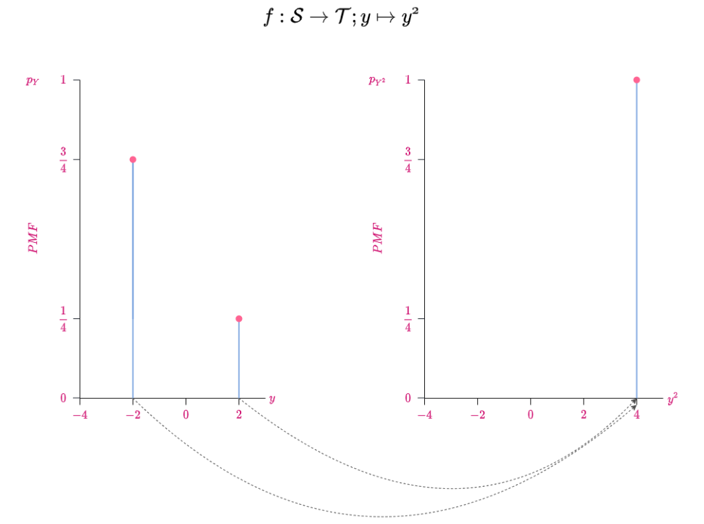
As is obvious from the diagrams, the probability distributions corresponding to the random variables X^2 \text{ and } Y^2 are the same. Hence their total variation distance will be zero. On the contrary, we can see that the probability distributions corresponding to the random variables X \text{ and } Y are different and hence their total variation distance will be some positive value. Therefore, the total variation distance between the random variables X^2 \text{ and } Y^2 is less than the total variation distance between the random variables X \text{ and } Y.
Let us now calculate the total variation distance between X^2 \text{ and } Y^2 and also the total variation distance between X \text{ and } Y and check whether our calculations match what we have proved. We will also get some practice in calculating total variation distance.😛
\begin{equation*}
\begin{split}
\big\|X - Y\big\|_{TV} & = \frac{1}{2}\underset{\mathcal{s \in S}}{\sum} \big|P(X = s) - P(Y = s) \big| \\
& = \frac{1}{2}\bigg[\Big|P(X = -2) - P(Y = -2)  \Big| + \Big|P(X = 2) - P(Y = 2)  \Big| \bigg] \\
& = \frac{1}{2}\bigg[\Big|\frac{1}{4} - \frac{3}{4}  \Big| + \Big|\frac{3}{4} - \frac{1}{4}  \Big| \bigg] \\
& = \frac{1}{2}\bigg[\frac{1}{2}+ \frac{1}{2} \bigg] \\
& = \frac{1}{2}
\end{split}
\end{equation*}
Just for practice let us also calculate total variation distance between random variables X \text{ and } Y using an alternate definition.
Let \mathcal{A = \big\{s \in S : } \, P(X = s) \geq P(Y = s)\big\}. From the probability distributions corresponding to random variables X \text{ and } Y, we see that \mathcal{A = \{2\}}.
\begin{equation*}
\begin{split}
\big\|X - Y\big\|_{TV} & = \big|P(X \in \mathcal{A}) - P(Y \in \mathcal{A})\big| \\
& =  \big| P(X = 2) - P(Y = 2) \big| \\
& = \bigg|\frac{3}{4} - \frac{1}{4}\bigg| \\
& = \frac{1}{2}
\end{split}
\end{equation*}
We have already proved that \big\|X - Y\big\|_{TV} = \big|P(X \in \mathcal{A}) - P(Y \in \mathcal{A})\big| = \big|P(X \in \mathcal{A^c}) - P(Y \in \mathcal{A^c})\big|. Let us verify this through calculation.
Since \mathcal{A = \{2\} \text{ , } A^c = \{-2\}}.
Hence, \big|P(X \in \mathcal{A^c}) - P(Y \in \mathcal{A^c})\big| = \big|P(X = -2) - P(Y = -2)\big| = \big|\frac{1}{4} - \frac{3}{4}\big| = \frac{1}{2}.
So we have verified that \big\|X - Y\big\|_{TV} = \big|P(X \in \mathcal{A}) - P(Y \in \mathcal{A})\big| = \big|P(X \in \mathcal{A^c}) - P(Y \in \mathcal{A^c})\big| = \frac{1}{2}.
We see that both the definitions of total variation distance between two random variables yield the same results.
\begin{equation*}
\begin{split}
\big\|f(X) - f(Y)\big\|_{TV} & = \frac{1}{2}\underset{\mathcal{t \in T}}{\sum} \big|P(X = t) - P(Y = t) \big| \\
& = \frac{1}{2} \bigg|P(X = 4) - P(Y = 4) \bigg| \\
& = \frac{1}{2} \bigg|1 - 1 \bigg| \\
& = 0
\end{split}
\end{equation*}
Since \big\|X - Y\big\|_{TV} = \frac{1}{2} \text{ and } \big\|f(X) - f(Y)\big\|_{TV} = 0, \big\|f(X) - f(Y)\big\|_{TV} < \big\|X - Y\big\|_{TV}.
Now consider the function \mathcal{f : S \rightarrow T; z \mapsto z + 2}. The set \mathcal{S = \{-2, 2\}} and the probability distributions corresponding to random variables X \text{ and } Y are the same as in the previous example.
The set \mathcal{T = \{0, 4\}}.
Also, f(X) = X + 2 \text{ and } f(Y) = Y + 2.
Since \mathcal{T} is the support of random variables X + 2 \text{ and } Y + 2,
X + 2 = \{0, 4\} \text{ and } Y + 2 = \{0, 4\}.
The probability distributions corresponding to random variables X + 2 \text{ and } Y + 2 are as follows:
p_{X + 2}(0) = P(X + 2 = 0) = P(X = -2) = \frac{1}{4} \text{ , } p_{X + 2}(4) = P(X + 2 = 4) = P(X = 2) = \frac{3}{4} and
p_{Y + 2}(0) = P(Y + 2 = 0) = P(Y = -2) = \frac{3}{4} \text{ , } p_{Y + 2}(4) = P(Y + 2 = 4) = P(Y = 2) = \frac{1}{4}.
The following is a pictorial representation of the probability distributions corresponding to the random variables X, X +2, Y, Y + 2.


We can see that the probability distribution corresponding to random variable X is the same as that corresponding to random variable X + 2. Similarly for Y \text{ and } Y + 2. Since the function f does not change the distribution, \big\|f(X) - f(Y)\big\|_{TV} = \big\|X - Y\big\|_{TV}.
So for the function \mathcal{f : S \rightarrow T ; z \mapsto z^2} \text{ , } \big\|f(X) - f(Y)\big\|_{TV} < \big\|X - Y\big\|_{TV} and for the function \mathcal{f : S \rightarrow T ; z \mapsto z + 2} \text{ , } \big\|f(X) - f(Y)\big\|_{TV} = \big\|X - Y\big\|_{TV}.
Hence \big\|f(X) - f(Y)\big\|_{TV} \leq \big\|X - Y\big\|_{TV}.
Wakey-wakey! In case you slept through the discussion,😴, now is the time to be alert and do some exercises to test your understanding.
Examples of Total Variation Distance Calculation
Exercise 1
Let X \text{ and } Y be independent random variables, each uniformly distributed over \mathbb{Z}_p, where p is prime. Calculate \big\|(X, Y) - (X, XY)\big\|_{TV}.
Before we calculate the total variation distance, now would be a good time to refresh some concepts in probability namely, joint distribution and independence of random variables and conditional independence of random variables.
Let \mathcal{S = \{(x, y) : x, y \in \mathbb{Z}_p \text{, where } p \text{ is prime}\}}.
By definition,
\big\|(X, Y) - (X, XY)\big\|_{TV} = \frac{1}{2} \sum_{(x, y)\, \in \, \mathcal{S}} \big|P(X = x, Y = y) - P(X = x, XY = xy)\big|In order to calculate the total variation distance we would first need to construct the PMFs of the random variables X, Y, (X, Y) \text{ and }(X, XY).
Since X \text{ and }Y are uniformly distributed over the set of all prime numbers,
p_X(x) = P(X = x) = \frac{1}{\big|\mathbb{Z_p}\big|} \text{ and } p_Y(y) = P(Y = y) = \frac{1}{\big|\mathbb{Z_p}\big|}, for all x, y \in \mathbb{Z_p}.
p_{X, Y}(x, y) = P(X = x, Y = y) = P(X = x) P(Y=y) = \frac{1}{\big|\mathbb{Z_p}\big|} \times \frac{1}{\big|\mathbb{Z_p}\big|} = \frac{1}{{\big|\mathbb{Z_p}\big|}^2} , for all x, y \in \mathbb{Z_p}.
In the above equation, P(X = x, Y = y) = P(X = x) P(Y=y) because X \text{ and }Y are independent.
\begin{equation*}
\begin{split}
p_{X, XY}(x, xy) & = P(X = x, XY = xy) \text{ (for all } x, y \in \mathbb{Z_p} )\\
& = P(X = x) P(XY = xy \,|\, X = x) \\
& = P(X = x) P(X = x, Y = y \,|\, X = x) \\
& = P(X = x) P(X = x \,|\, X = x) P(Y = y \,|\, X = x) \text{ (since } X \text{ and } Y \text{ are independent)}\\
& = \frac{1}{\big|\mathbb{Z_p}\big|} \times 1 \times P(Y = y) \text{ (since } X \text{ and } Y \text{ are independent)}\\
& = \frac{1}{\big|\mathbb{Z_p}\big|} \times 1 \times \frac{1}{\big|\mathbb{Z_p}\big|} \\
& = \frac{1}{{\big|\mathbb{Z_p}\big|}^2} \\
\end{split}
\end{equation*}
Hence,
\begin{equation*}
\begin{split}
\big\|(X, Y) - (X, XY)\big\|_{TV} & = \frac{1}{2} \sum_{(x, y)\, \in \, \mathcal{S}} \big|P(X = x, Y = y) - P(X = x, XY = xy)\big| \\
& = \frac{1}{2} \sum_{(x, y)\, \in \, \mathcal{S}} \Bigg|\frac{1}{{\big|\mathbb{Z_p}\big|}^2} - \frac{1}{{\big|\mathbb{Z_p}\big|}^2}\Bigg| \\
& = 0.
\end{split}
\end{equation*}
Intuitively this makes sense because the distribution of (X, XY) has no new information compared to the distribution of (X, Y), hence they resolve into identical distributions.
Lets do one more example before wrapping up the discussion on total variation distance.
Exercise 2
Let X \text{ and } Y be discrete random variables, each taking values in the interval [0..r] (when r is an integer; the notation [0..r] denotes the interval of all integers between 0 \text{ and } r with 0 \text{ and } r included). Show that \big|E[X] - E[Y]\big| \leq 2r \big\|X - Y \big\|_{TV}.
Before we do this exercise, if you need to refresh your understanding of expectation, you can refer here.
By definition,
E(X) = \overset{r}{\underset{i = 0}{\sum}} \,i \,P(X = i) \text{ and } E(Y) = \overset{r}{\underset{i = 0}{\sum}} \,i \,P(Y = i).
\begin{equation*}
\begin{split}
\big|E(X) - E(Y)\big| & = \Big|\sum_{i = 0}^{r} i\, P(X = i) - \sum_{i = 0}^{r} i \,P(Y = i)\Big| \\
& = \Big|\sum_{i = 0}^{r} i \big[P(X = i) - P(Y = i)\big]\Big| \\
& \leq \sum_{i = 0}^{r} i \Big| \big[P(X = i) - P(Y = i)\big]\Big| \\
& \leq r \sum_{i = 0}^{r} \Big| \big[P(X = i) - P(Y = i)\big]\Big| \\
& \leq 2r \big\|X - Y \big\|_{TV} \\
& \leq r \big\|X - Y \big\|_1 \\
\end{split}
\end{equation*}
For a summary of all the results we have proved so far refer here.
Now that we have an in depth understanding of total variation distance, distinguishing advantage, distinguishing distance and bias, let us use these concepts to calculate the advantage of an adversary with respect to a challenger i.e., the distinguishing advantage in a game played between them. This exercise will serve as a warmup before doing security proofs in cryptography. Security proofs use mathematics to reason about the security of cryptographic systems. They are the building blocks for constructing secure cryptographic systems.