authored by Premmi and Beguène
In Simple Settings
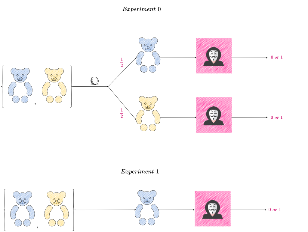
Annie is on her summer vacation and she decides to take a break from reading. Her neighbor Marie is her nemesis and so Annie devises a game to outsmart her. Annie has two bears, one blue and the other yellow. Annie’s game is as follows:
She devises two experiments – Experiment \textit{0} and Experiment \textit{1}.
In Experiment \textit{0}, Annie randomly picks a bear, with each bear having equal probability of being picked. She communicates to Marie the color of the bear she picked.
In Experiment \textit{1}, Annie always picks the blue bear and communicates the color ‘Blue’ to Marie.
Marie’s goal is to distinguish Experiment \textit{0} from Experiment \textit{1}. At the end of each experiment (i.e., when Marie receives a color from Annie), she outputs 0 or 1 as a guess for which experiment she thinks she is in. She wins if she guesses correctly, otherwise she loses.
They play this game several times.
The following diagram is a pictorial representation of the two experiments.
To distinguish between the two experiments, Marie has to maximize her distinguishing advantage. How does she do that?
Before proceeding, let us define some notations we will be using.
Let \mathcal{S = \{\textit{'Blue', 'Yellow'}\}} denote the sample space which comprises the possible outcomes of the experiments 0 \text{ and } 1.
Let E_0 \text{ and } E_1 be random variables denoting the outcome of experiments 0 \text{ and } 1 respectively.
We know that a random variable maps the sample space to a real line i.e., ‘Blue’ would be mapped to a real number and ‘Yellow’ would be mapped to another real number. But for clarity’s sake we will omit this mapping and directly deal with the values in the sample space, \mathcal{S}.
Suppose say ‘Blue’ maps to 1, then P(E_0 = 1) would denote the probability that the outcome of experiment 0 is 1 i.e., ‘Blue’ (Annie picks a ‘Blue’ bear and communicates the color ‘Blue’ to Marie). We would instead denote this probability as P(E_0 = \textit{'Blue'}), for ease of understanding.
For Marie to win, she needs to distinguish between experiments 0 \text{ and } 1. Her success in distinguishing between the two experiments depends on how different the outcomes of the two experiments are. For example, if she gets ‘Yellow’ she knows that it is the outcome of experiment 0 since it is impossible for experiment 1 to have an outcome of ‘Yellow’.
Hence her success in distinguishing between the two experiments depends on how different the probability distributions of the outcomes of the two experiments are i.e., the distance (to be precise, the total variation distance) between the distributions of E_0 \text{ and } E_1 and her ability to measure this distance accurately.
Therefore, to distinguish between experiment 0 \text{ and } 1, she tries to maximize her distinguishing advantage (or equivalently, the distinguishing distance), namely the quantity,
\big|P[\mathcal{D}(E_0) = 1] - P[\mathcal{D}(E_1) = 1]\big|where \mathcal{D(\cdot)} is a distinguisher function that distinguishes between the probability distributions of E_0 \text{ and } E_1. \mathcal{D}(E_0) means \mathcal{D} takes as input \mathcal{s \in S}, where \mathcal{s} is drawn from the distribution of E_0 and outputs either 0 or 1. Similarly for \mathcal{D}(E_1). This quantity is denoted by \text{Adv}_D(E_0, E_1).
We have already proved that,
\big\|E_0 - E_1\big\|_{TV} = \underset{\mathcal{D : S \rightarrow \{0, 1\}}}{\text{max}} \big|P[\mathcal{D}(E_0) = 1] - P[\mathcal{D}(E_1) = 1]\big|where \big\|E_0 - E_1\big\|_{TV} is the total variation distance between the probability distributions of random variables E_0 \text{ and } E_1 i.e., the probability distributions of the outcomes of experiments 0 \text{ and } 1.
From this equation, we can infer that the total variation distance between the distributions of E_0 \text{ and } E_1 maximizes the distinguishing advantage.
An alternate way to express the above equation is as follows,
\big\|E_0 - E_1\big\|_{TV} = \underset{\mathcal{A : S \rightarrow \{0, 1\}}}{\text{max}} \mathcal{\big|P[\mathcal{W_0}] - P[\mathcal{W_1}]\big|}where \mathcal{W_0} is the event that the adversary \mathcal{A} (Marie) outputs \mathcal{1} when given as input \mathcal{s \in S} drawn from the distribution of E_0 and \mathcal{W_1} is the event that the adversary \mathcal{A} outputs \mathcal{1} when given as input \mathcal{s \in S} drawn from the distribution of E_1.
Or expressed more succinctly, W_b is the event that Marie outputs 1 in experiment b, where b = \{0, 1\}.
We have also already proved that,
\big\|E_0 - E_1\big\|_{TV} = \frac{1}{2} \Big\|E_0 - E_1\Big\|_1 = \frac{1}{2}\underset{\mathcal{s \in S}}{\sum} \big|P(E_0 = s) - P(E_1 = s) \big|Since the total variation distance between random variables E_0 \text{ and } E_1 maximizes the distinguishing advantage, in order to calculate this distance we need to construct the probability distributions of E_0 \text{ and } E_1.
The PMF of E_0, p_{E_0}, is given by,
\begin{equation*}
\begin{split}
p_{E_0}(\textit{'Blue'}) & = P(E_0 = \textit{'Blue'}) = \frac{1}{2} \\
p_{E_0}(\textit{'Yellow'}) & = P(E_0 = \textit{'Yellow'}) = \frac{1}{2} \\
\end{split}
\end{equation*}
The PMF of E_1, p_{E_1}, is given by,
\begin{equation*}
\begin{split}
p_{E_1}(\textit{'Blue'}) & = P(E_1 = \textit{'Blue'}) = 1 \\
\end{split}
\end{equation*}
Therefore,
\begin{equation*}
\begin{split}
 \big\|E_0 - E_1\big\|_{TV} & = \frac{1}{2}\underset{\mathcal{s \in S}}{\sum} \big|P(E_0 = s) - P(E_1 = s) \big| \\
& = \frac{1}{2} \bigg[\Big|P(E_0 = \textit{'Blue'}\,) - P(E_1 = \textit{'Blue'}\,) \Big| + \Big|P(E_0 = \textit{'Yellow'}\,) - P(E_1 = \textit{'Yellow'}\,) \Big|\bigg] \\
& = \frac{1}{2}\Bigg[\bigg|\frac{1}{2} - 1\bigg| + \bigg|\frac{1}{2} - 0\bigg|\Bigg] \\
& = \frac{1}{2} \\
\end{split}
\end{equation*}
This shows that the maximum advantage possible in distinguishing between the two experiments is \frac{1}{2}. Since Marie’s distinguishing advantage is due to the difference in probability distributions of the outcomes of the experiments, her distinguishing advantage cannot be more than the total variation distance between the two distributions, which is a measure of the difference between the two distributions.
The following is a pictorial representation of the probability distributions of the outcomes of experiments 0 \text{ and } 1.

The following diagram shows an alternate way to calculate total variation distance between the outcomes of experiments 0 \text{ and } 1.

The total variation distance between distributions of random variables E_0 \text{ and } E_1 denoting the outcomes of experiments 0 \text{ and } 1 respectively, can also be defined as
\big\|E_0 - E_1\big\|_{TV} = \underset{\mathcal{B} \,\subset\, \mathcal{S}}{\text{max}} \big|P(E_0 \in \mathcal{B}) - P(E_1 \in \mathcal{B}) \big|We have already proved that both sets \mathcal{A = \{ s \in S :\, } P(E_0 = s) \geq P(E_1 = s)\} and \mathcal{A^c = \{ s \in S :\, } P(E_0 = s) < P(E_1 = s)\} maximize \big|P(E_0 \in \mathcal{B}) - P(E_1 \in \mathcal{B}) \big|.
Here, \mathcal{A = \{\textit{'Yellow'}\}} and \mathcal{A^c = \{\textit{'Blue'}\}}. Also, the support of random variables E_0 \text{ and } E_1 is \{\textit{'Blue', 'Yellow'}\}.
Hence,
\begin{equation*}
\begin{split}
\big\|E_0 - E_1\big\|_{TV} & = \big|P(E_0 \in \mathcal{A}) - P(E_1 \in \mathcal{A}) \big| \\
& =  \bigg|\frac{1}{2} - 0\bigg| \\
& = \frac{1}{2} \\
\end{split}
\end{equation*}
Also,
\begin{equation*}
\begin{split}
\big\|E_0 - E_1\big\|_{TV} & = \big|P(E_0 \in \mathcal{A^c}) - P(E_1 \in \mathcal{A^c}) \big| \\
& =  \bigg|\frac{1}{2} - 1\bigg| \\
& = \frac{1}{2} \\
\end{split}
\end{equation*}
We have already proved that for any distinguisher \mathcal{D},
\text{Adv}_D(E_0, E_1) \leq \big\|E_0 - E_1\big\|_{TV}We have proved mathematically that Marie’s distinguishing advantage cannot be more than \frac{1}{2}. Marie’s distinguishing advantage depends on the distinguisher function that she uses to distinguish between the two distributions. In order for Marie to maximize her distinguishing advantage, she needs to find the best distinguisher function i.e., one that maximizes her advantage.
When Annie sends a color to Marie, how does Marie construct her distinguisher function so that she maximizes her distinguishing advantage?
Before we use mathematics to construct the required distinguisher function, let us use our intuition to think through this problem and then verify the soundness of our intuition mathematically.
Since distinguishing advantage is the absolute difference in probabilities between Marie winning and Marie losing i.e.,
\begin{equation*}
\begin{split}
\textit{Distinguishing Advantage} & = \big|\text{Advantage of adversary with respect to challenger}\big| \\
& = \big|P(\text{Adversary wins}) - P(\text{Challenger wins})\big| \\
& = \big|P(\text{Adversary wins}) - P(\text{Adversary loses})\big| \\
& = \big|P(\text{Marie wins}) - P(\text{Marie loses})\big| \\
\end{split}
\end{equation*}
in order for Marie to maximize her distinguishing advantage, she needs to maximize her probability of winning (which in turn minimizes her probability of losing).
How does she maximize her probability of winning? Since she can get two colors as input namely, ‘Blue’ and ‘Yellow’ she needs to maximize her probability of winning in each case. Lets examine the two cases.
- Marie gets ‘Yellow’ as input
Marie knows that she can get ‘Yellow’ as an outcome only in experiment \mathcal{0}. Hence she maximizes her probability of winning (her probability of winning is \mathcal{1}) by outputting \mathcal{0} whenever she gets ‘Yellow’ as input. - Marie gets ‘Blue’ as input
Marie can get ‘Blue’ as an outcome only both experiments i.e., in \mathcal{0 \text{ and } 1}. The probability that she gets ‘Blue’ is given by,
\begin{equation*}
\begin{split}
P(\textit{Blue}) & = P(\textit{Experiment }\mathcal{0})\times P(\textit{Blue | Experiment }\mathcal{0}) \\
& \,\,\,\,\,+ P(\textit{Experiment }\mathcal{1})\times P(\textit{Blue | Experiment }\mathcal{1})\\
& = \frac{1}{2} \times \frac{1}{2} + \frac{1}{2} \times 1 \\
& = \frac{1}{4} + \frac{1}{2}
\end{split}
\end{equation*}
So when Marie gets ‘Blue’, there is a \mathcal{\frac{1}{4}} \div \frac{3}{4} = \frac{1}{4} \times \frac{4}{3} = \frac{1}{3} probability that it comes from experiment \mathcal{0} and \mathcal{\frac{2}{3}} probability that it comes from experiment \mathcal{1}. So ‘Blue’ is twice more likely to be an outcome of experiment \mathcal{1} than \mathcal{0}. Since Marie wants to maximize her probability of winning, when she gets ‘Blue’ and outputs \mathcal{1}, she is twice more likely to be correct than wrong. Hence to maximize her probability of winning she should output \mathcal{1} when she gets ‘Blue’ as input.
By this reasoning, the best distinguisher i.e., the one that maximizes her distinguishing advantage outputs \mathcal{0} when given ‘Yellow’ as input and outputs \mathcal{1} when given ‘Blue’ as input.
Since distinguishing advantage is an absolute value i.e., it only measures the distinguishability between experiments, the inverse strategy should also work. So another distinguisher which would maximize her advantage would be one that outputs \mathcal{0} when given ‘Blue’ as input and outputs \mathcal{1} when given ‘Yellow’ as input.
Any other distinguisher would give a distinguishing advantage less than what the above two distinguishers would give.
To verify this hypothesis, let us construct the following two distinguisher functions and calculate the respective advantages that they give.
- Distinguisher function \mathcal{D} on getting ‘Blue’ as input outputs \mathcal{0} with probability \mathcal{\frac{1}{3}} and \mathcal{1} with probability \mathcal{\frac{2}{3}}.
Distinguisher function \mathcal{D} on getting ‘Yellow’ as input outputs \mathcal{0} with probability \mathcal{1}. - Distinguisher function \mathcal{D} on getting ‘Blue’ as input outputs \mathcal{0} with probability \mathcal{\frac{1}{2}} and \mathcal{1} with probability \mathcal{\frac{1}{2}}.
Distinguisher function \mathcal{D} on getting ‘Yellow’ as input outputs \mathcal{0} with probability \mathcal{1}.
If our reasoning is correct, the distinguishing advantage of the distinguisher described in \mathcal{(1)} will be more than that of distinguisher described in \mathcal{(2)}, since when Marie gets ‘Blue’ it is twice more likely to be the outcome of experiment \mathcal{1} than \mathcal{0}, any distinguisher that outputs \mathcal{1} with a higher probability when given ‘Blue’, will have a higher probability of winning. Hence the best distinguisher will output \mathcal{1} with probability \mathcal{1} when given ‘Blue’ as input. Since distinguisher in \mathcal{(1)} outputs \mathcal{1} with probability \mathcal{\frac{2}{3}} when given ‘Blue’ as input and distinguisher in \mathcal{(2)} outputs \mathcal{1} with probability \mathcal{\frac{1}{2}} when given ‘Blue’ as input, the distinguishing advantage we get using distinguisher in \mathcal{(1)} will be more than what we get when using distinguisher in \mathcal{(2)} \big(since ‘Blue’ occurs twice more times in experiment \mathcal{1} than \mathcal{0} and \mathcal{\frac{2}{3} > \frac{1}{2}}\big).
Let us enumerate the distinguishers we have come up with so far through our reasoning. We will calculate the distinguishing advantage of each of these distinguishers and use the definition of distinguishing advantage (which we have derived earlier) to check whether our reasoning is correct.
Since Marie can get either of ‘Blue’ or ‘Yellow’ as input,
P(\textit{'Blue'}) + P(\textit{'Yellow'}) = 1We have already calculated P(\textit{'Blue'}) = \frac{3}{4}. Of the \frac{3}{4} times ‘Blue’ occurs \frac{1}{4} is from experiment \mathcal{0} and \frac{1}{2} is from experiment \mathcal{1}. Also,
\begin{equation*}
\begin{split}
P(\textit{'Yellow'}) & = P(\textit{'Experiment 0'})\, P(\textit{'Yellow'}\, | \textit{'Experiment 0'}) \\
& \,\,\,\,\,\,+ P(\textit{'Experiment 1'}) \,P(\textit{'Yellow'} \,| \textit{'Experiment 1'}) \\
& = \frac{1}{2} \times \frac{1}{2} + \frac{1}{2} \times 0 \\
& = \frac{1}{4} \\
\end{split}
\end{equation*}
Another equivalent way to calculate P(\textit{'Yellow'}) is,
P(\textit{'Yellow'}) = 1 - P(\textit{'Blue'}) = 1 - \frac{3}{4} = \frac{1}{4}.
Let us calculate the distinguishing advantage of each of the distinguishers we have described so far.The distinguisher function \mathcal{D} outputs \mathcal{0} on getting ‘Yellow’ as input and outputs \mathcal{1} on getting ‘Blue’ as input.
By definition,
\textit{Distinguishing Advantage} = \big|P(\text{Marie wins}) - P(\text{Marie loses})\big|.
\begin{equation*}
\begin{split}
\hspace*{0.4cm} P(\text{Marie Wins}) & = P(\textit{Experiment 0})\, P(\text{Marie Wins}\, | \textit{Experiment 0}) \\
& \,\,\,\,\,\,+ P(\textit{Experiment 1})\, P(\text{Marie Wins}\, | \textit{Experiment 1}) \\
& = P(\textit{Experiment 0})\, \Bigg[ P(\textit{'Blue'} \, | \textit{Experiment 0}) P(\text{Marie Wins} \, | \textit{'Blue'} \text{ and } \textit{Experiment 0}) \\
& \hspace*{3.2cm} + P(\textit{'Yellow'} \, | \textit{Experiment 0}) P(\text{Marie Wins} \, | \textit{'Yellow'} \text{ and } \textit{Experiment 0}) \Bigg] \\
& \hspace*{0.4cm}+ P(\textit{Experiment 1})\, \Bigg[ P(\textit{'Blue'} \, | \textit{Experiment 1}) P(\text{Marie Wins} \, | \textit{'Blue'} \text{ and } \textit{Experiment 1}) \\
& \hspace*{3.6cm} + P(\textit{'Yellow'} \, | \textit{Experiment 1}) P(\text{Marie Wins} \, | \textit{'Yellow'} \text{ and } \textit{Experiment 1}) \Bigg] \\
& = \frac{1}{2} \Bigg[ \frac{1}{2} \times 0 + \frac{1}{2} \times 1 \Bigg] + \frac{1}{2} \Bigg[ 1 \times 1 + 0 \times 0\Bigg] \\
& = \frac{1}{2} \Bigg[\frac{1}{2}\Bigg] +  \frac{1}{2} \\
& = \frac{3}{4} \\
P(\text{Marie Loses}) & = 1 - P(\text{Marie Wins}) \\
& = 1 - \frac{3}{4} \\
& = \frac{1}{4} \\
\hspace*{0.6cm} \textit{Distinguishing Advantage} & = \big|P(\text{Marie wins}) - P(\text{Marie loses})\big| \\
& = \Bigg|\frac{3}{4} - \frac{1}{4}\Bigg| \\
& = \frac{1}{2} \\
\end{split}
\end{equation*}
Since we have already proved that the distinguishing advantage cannot be greater than \frac{1}{2}, this confirms that our reasoning is correct, i.e., this distinguishing function \mathcal{D} is the best possible distinguisher.
Next lets calculate the distinguishing advantage of a distinguisher that does the inverse of the previous distinguisher, namely outputs 1 when it gets ‘Yellow’ as input and outputs 0 when it gets ‘Blue’ as input.
\begin{equation*}
\begin{split}
P(\text{Marie Wins}) & = P(\textit{Experiment 0})\, P(\text{Marie Wins}\, | \textit{Experiment 0}) \\
& \,\,\,\,\,\,+ P(\textit{Experiment 1})\, P(\text{Marie Wins}\, | \textit{Experiment 1}) \\
& = P(\textit{Experiment 0})\, \Bigg[ P(\textit{'Blue'} \, | \textit{Experiment 0}) P(\text{Marie Wins} \, | \textit{'Blue'} \text{ and } \textit{Experiment 0}) \\
& \hspace*{3.2cm} + P(\textit{'Yellow'} \, | \textit{Experiment 0}) P(\text{Marie Wins} \, | \textit{'Yellow'} \text{ and } \textit{Experiment 0}) \Bigg] \\
& \hspace*{0.4cm}+ P(\textit{Experiment 1})\, \Bigg[ P(\textit{'Blue'} \, | \textit{Experiment 1}) P(\text{Marie Wins} \, | \textit{'Blue'} \text{ and } \textit{Experiment 1}) \\
& \hspace*{3.6cm} + P(\textit{'Yellow'} \, | \textit{Experiment 1}) P(\text{Marie Wins} \, | \textit{'Yellow'} \text{ and } \textit{Experiment 1}) \Bigg] \\
& = \frac{1}{2} \Bigg[ \frac{1}{2} \times 1 + \frac{1}{2} \times 0 \Bigg] + \frac{1}{2} \Bigg[ 1 \times 0 + 0 \times 0\Bigg] \\
& = \frac{1}{4} \\
P(\text{Marie Loses}) & = 1 - P(\text{Marie Wins}) \\
& = \frac{3}{4} \\
\textit{Distinguishing Advantage} & = \big|P(\text{Marie wins}) - P(\text{Marie loses})\big| \\
& = \Bigg|\frac{1}{4} - \frac{3}{4}\Bigg| \\
& = \frac{1}{2} \\
\end{split}
\end{equation*}
We had already reasoned that this distinguisher will also maximize the distinguishing advantage because it maximizes the probability of losing and consequently minimizes the probability of winning. Since distinguishing advantage is an absolute value, this distinguisher is equivalent to one that maximizes the probability of winning and consequently minimizes the probability of losing. Hence both the distinguishers have the same distinguishing advantage of \frac{1}{2} as can be seen for the calculations.
Now lets calculate the distinguishing advantage of a distinguisher \mathcal{D} that on getting ‘Yellow’ as input, outputs \mathcal{0} with probability \mathcal{1} and on getting ‘Blue’ as input, outputs \mathcal{0} with probability \mathcal{\frac{1}{3}} and \mathcal{1} with probability \mathcal{\frac{2}{3}}.
\begin{equation*}
\begin{split}
\hspace*{0.4cm} P(\text{Marie Wins}) & = P(\textit{Experiment 0})\, P(\text{Marie Wins}\, | \textit{Experiment 0}) \\
& \,\,\,\,\,\,+ P(\textit{Experiment 1})\, P(\text{Marie Wins}\, | \textit{Experiment 1}) \\
& = P(\textit{Experiment 0})\, \Bigg[ P(\textit{'Blue'} \, | \textit{Experiment 0}) P(\text{Marie Wins} \, | \textit{'Blue'} \text{ and } \textit{Experiment 0}) \\
& \hspace*{3.2cm} + P(\textit{'Yellow'} \, | \textit{Experiment 0}) P(\text{Marie Wins} \, | \textit{'Yellow'} \text{ and } \textit{Experiment 0}) \Bigg] \\
& \hspace*{0.4cm}+ P(\textit{Experiment 1})\, \Bigg[ P(\textit{'Blue'} \, | \textit{Experiment 1}) P(\text{Marie Wins} \, | \textit{'Blue'} \text{ and } \textit{Experiment 1}) \\
& \hspace*{3.6cm} + P(\textit{'Yellow'} \, | \textit{Experiment 1}) P(\text{Marie Wins} \, | \textit{'Yellow'} \text{ and } \textit{Experiment 1}) \Bigg] \\
& = \frac{1}{2} \Bigg[ \frac{1}{2} \times \frac{1}{3} + \frac{1}{2} \times 1 \Bigg] + \frac{1}{2} \Bigg[ 1 \times \frac{2}{3} + 0 \times 0\Bigg] \\
& = \frac{1}{2} \Bigg[\frac{1}{6} + \frac{1}{2} \Bigg] +  \frac{1}{3} \\
& = \frac{1}{2} \Bigg[\frac{4}{6} \Bigg] +  \frac{1}{3} \\
& = \frac{2}{3} \\
P(\text{Marie Loses}) & = 1 - P(\text{Marie Wins}) \\
& = 1 - \frac{2}{3} \\
& = \frac{1}{3} \\
\hspace*{0.6cm} \textit{Distinguishing Advantage} & = \big|P(\text{Marie wins}) - P(\text{Marie loses})\big| \\
& = \Bigg|\frac{2}{3} - \frac{1}{3}\Bigg| \\
& = \frac{1}{3} \\
\end{split}
\end{equation*}
We have already discussed why the distinguishing advantage of this distinguisher must be less than the previous two distinguishers and the above calculation confirms that our reasoning is correct.
Now let us calculate the distinguishing advantage of a distinguisher that we reasoned will perform worse than previous distinguisher and verify whether this indeed is the case.
Distinguisher function \mathcal{D} on getting ‘Yellow’ as input, outputs \mathcal{0} with probability \mathcal{1} and on getting ‘Blue’ as input outputs \mathcal{0} with probability \mathcal{\frac{1}{2}} and \mathcal{1} with probability \mathcal{\frac{1}{2}}.
\begin{equation*}
\begin{split}
\hspace*{0.4cm} P(\text{Marie Wins}) & = P(\textit{Experiment 0})\, P(\text{Marie Wins}\, | \textit{Experiment 0}) \\
& \,\,\,\,\,\,+ P(\textit{Experiment 1})\, P(\text{Marie Wins}\, | \textit{Experiment 1}) \\
& = P(\textit{Experiment 0})\, \Bigg[ P(\textit{'Blue'} \, | \textit{Experiment 0}) P(\text{Marie Wins} \, | \textit{'Blue'} \text{ and } \textit{Experiment 0}) \\
& \hspace*{3.2cm} + P(\textit{'Yellow'} \, | \textit{Experiment 0}) P(\text{Marie Wins} \, | \textit{'Yellow'} \text{ and } \textit{Experiment 0}) \Bigg] \\
& \hspace*{0.4cm}+ P(\textit{Experiment 1})\, \Bigg[ P(\textit{'Blue'} \, | \textit{Experiment 1}) P(\text{Marie Wins} \, | \textit{'Blue'} \text{ and } \textit{Experiment 1}) \\
& \hspace*{3.6cm} + P(\textit{'Yellow'} \, | \textit{Experiment 1}) P(\text{Marie Wins} \, | \textit{'Yellow'} \text{ and } \textit{Experiment 1}) \Bigg] \\
& = \frac{1}{2} \Bigg[ \frac{1}{2} \times \frac{1}{2} + \frac{1}{2} \times 1 \Bigg] + \frac{1}{2} \Bigg[ 1 \times \frac{1}{2} + 0 \times 0\Bigg] \\
& = \frac{1}{2} \Bigg[\frac{3}{4} \Bigg] +  \frac{1}{4} \\
& = \frac{3}{8} +  \frac{1}{4} \\
& = \frac{5}{8} \\
P(\text{Marie Loses}) & = 1 - P(\text{Marie Wins}) \\
& = 1 - \frac{5}{8} \\
& = \frac{3}{8} \\
\hspace*{0.6cm} \textit{Distinguishing Advantage} & = \big|P(\text{Marie wins}) - P(\text{Marie loses})\big| \\
& = \Bigg|\frac{5}{8} - \frac{3}{8}\Bigg| \\
& = \frac{1}{4} \\
\end{split}
\end{equation*}
As expected the distinguishing advantage of this distinguisher is less than that of the previous distinguisher.
These calculations confirm that to maximize the distinguishing advantage we have to design the distinguisher in such a way that it maximizes Marie’s (adversary’s) probability of winning.
Now let us come up with the best distinguisher using mathematics and show that it would be the same distinguishers we arrived at using our reasoning.
By definition,
\begin{equation*}
\begin{split}
\textit{Distinguishing Advantage} & = \big|\text{Advantage of adversary with respect to challenger}\big| \\
& = \big|P(\text{Adversary wins}) - P(\text{Challenger wins})\big| \\
& = \big|P(\text{Adversary wins}) - P(\text{Adversary loses})\big| \\
& \,\,\,\vdots \\
& = \big|P[\mathcal{D}(E_0) = 1] - P[\mathcal{D}(E_1) = 1]\big| \\
\end{split}
\end{equation*}
Marie, in order to maximize her distinguishing advantage should find a distinguisher function \mathcal{D}(\cdot) that maximizes \big|P[\mathcal{D}(E_0) = 1] - P[\mathcal{D}(E_1) = 1]\big|.
She can maximize her distinguishing advantage in the following four ways :
- In order to maximize the difference \big|P[\mathcal{D}(E_0) = 1] - P[\mathcal{D}(E_1) = 1]\big|, Marie minimizes P[\mathcal{D}(E_1) = 1] and checks what is the maximum value P[\mathcal{D}(E_0) = 1] can take.
Since Marie tries to minimize P[\mathcal{D}(E_1) = 1] and the minimum value it can take is 0,
let P[\mathcal{D}(E_1) = 1] = 0.
P[\mathcal{D}(E_1) = 1] = 0 when the distinguisher outputs 0 when it gets ‘Blue’ as input.
When the distinguisher gets ‘Yellow’ as input, it can either output 0 \text{ or } 1. Let us see what happens in each case.
(i) Distinguisher outputs 0 when it gets ‘Yellow’ as input.
P[\mathcal{D}(E_0) = 1] = \frac{1}{2} \times 0 + \frac{1}{2} \times 0 = 0.
P[\mathcal{D}(E_0) = 1] is the probability that the distinguisher outputs 1, given an input (or sample drawn) from experiment 0. Since this distinguisher always outputs 0, irrespective of whether it gets ‘Blue’ or ‘Yellow’ as input, P[\mathcal{D}(E_0) = 1] = 0 \big(The factor of \frac{1}{2} is due to experiment 0 getting ‘Blue’ with probability \frac{1}{2} and ‘Yellow’ also with probability \frac{1}{2}\big).
Hence,
\textit{Distinguishing Advantage}, \text{Adv}_D(E_0, E_1) = \big|P[\mathcal{D}(E_0) = 1] - P[\mathcal{D}(E_1) = 1]\big| = \big| 0 - 0\big| = 0.
The distinguishing advantage of a distinguisher that always outputs 0 is 0.
(ii) Distinguisher outputs 1 when it gets ‘Yellow’ as input.
P[\mathcal{D}(E_0) = 1] = \frac{1}{2} \times 0 + \frac{1}{2} \times 1 = \frac{1}{2}.
Hence,
\textit{Distinguishing Advantage}, \text{Adv}_D(E_0, E_1) = \big|P[\mathcal{D}(E_0) = 1] - P[\mathcal{D}(E_1) = 1]\big| = \big| \frac{1}{2} - 0\big| = \frac{1}{2}.
The distinguishing advantage of a distinguisher that outputs 0 when given ‘Blue’ as input and 1 when given ‘Yellow’ as input is \frac{1}{2}. - In order to maximize the difference \big|P[\mathcal{D}(E_0) = 1] - P[\mathcal{D}(E_1) = 1]\big|, Marie maximizes P[\mathcal{D}(E_1) = 1] and checks what is the minimum value P[\mathcal{D}(E_0) = 1] can take.
Since Marie tries to maximize P[\mathcal{D}(E_1) = 1] and the maximum value it can take is 1, let P[\mathcal{D}(E_1) = 1] = 1.
P[\mathcal{D}(E_1) = 1] = 1 when the distinguisher outputs 1 when it gets ‘Blue’ as input.
When the distinguisher gets ‘Yellow’ as input, it can either output 0 \text{ or } 1. Let us see what happens in each case.
(i) Distinguisher outputs 0 when it gets ‘Yellow’ as input.
P[\mathcal{D}(E_0) = 1] = \frac{1}{2} \times 1 + \frac{1}{2} \times 0 = \frac{1}{2}.
Hence,
\textit{Distinguishing Advantage}, \text{Adv}_D(E_0, E_1) = \big|P[\mathcal{D}(E_0) = 1] - P[\mathcal{D}(E_1) = 1]\big| = \big| \frac{1}{2} - 1\big| = \frac{1}{2}.
The distinguishing advantage of a distinguisher that outputs 1 when given ‘Blue’ as input and 0 when given ‘Yellow’ as input is \frac{1}{2}.
(ii) Distinguisher outputs 1 when it gets ‘Yellow’ as input.
P[\mathcal{D}(E_0) = 1] = \frac{1}{2} \times 1 + \frac{1}{2} \times 1 = 1.
\textit{Distinguishing Advantage}, \text{Adv}_D(E_0, E_1) = \big|P[\mathcal{D}(E_0) = 1] - P[\mathcal{D}(E_1) = 1]\big| = \big| 1 - 1\big| = 0.
The distinguishing advantage of a distinguisher that always outputs 1 is 0. - In order to maximize the difference \big|P[\mathcal{D}(E_0) = 1] - P[\mathcal{D}(E_1) = 1]\big|, Marie minimizes P[\mathcal{D}(E_0) = 1] and checks what is the maximum value P[\mathcal{D}(E_1) = 1] can take.
Since Marie tries to minimize P[\mathcal{D}(E_0) = 1] and the minimum value it can take is 0, let P[\mathcal{D}(E_0) = 1] = 0.
P[\mathcal{D}(E_0) = 1] = 0 when the distinguisher always outputs 0. This is the distinguisher we have discussed in (1) (i) and its distinguishing advantage is 0. - In order to maximize the difference \big|P[\mathcal{D}(E_0) = 1] - P[\mathcal{D}(E_1) = 1]\big|, Marie maximizes P[\mathcal{D}(E_0) = 1] and checks what is the minimum value P[\mathcal{D}(E_1) = 1] can take.
Since Marie tries to maximize P[\mathcal{D}(E_0) = 1] and the maximum value it can take is 1, let P[\mathcal{D}(E_0) = 1] = 1.
P[\mathcal{D}(E_0) = 1] = 1 when the distinguisher always outputs 1. This is the distinguisher we have discussed in (2) (ii) and its distinguishing advantage is 0.
The distinguishers that maximize the distinguishing advantage are the ones in the cases (1) (ii) \text{ and } (2) (i). These are the same distinguishers we came up with through our reasoning.
Let us use the alternate notation used in defining distinguishing advantage and come up with the best distinguisher. Obviously this definition would also give us the same distinguishers we had already come up with. Let us do this exercise to convince ourselves that the two definitions are indeed equivalent (we have already proved their equivalence mathematically) and also more importantly so that we are fluent in using both these definitions.
Since we have already expounded on how to come up with the best distinguisher, this discussion will be succinct.
By definition,
\begin{equation*}
\begin{split}
\textit{Distinguishing Advantage} & = \big|\text{Advantage of adversary with respect to challenger}\big| \\
& = \big|P(\text{Adversary wins}) - P(\text{Challenger wins})\big| \\
& = \big|P(\text{Adversary wins}) - P(\text{Adversary loses})\big| \\
& \,\,\,\vdots \\
& = \mathcal{\big|P[\mathcal{W_0}] - P[\mathcal{W_1}]\big|}\\
\end{split}
\end{equation*}
where W_b is the event that Marie outputs 1 in experiment b, where b = \{0, 1\}.
As already discussed, we can maximize the distinguishing advantage, \mathcal{\big|P[\mathcal{W_0}] - P[\mathcal{W_1}]\big|} in four ways.
- In order to maximize the distinguishing advantage, \mathcal{\big|P[\mathcal{W_0}] - P[\mathcal{W_1}]\big|}, Marie minimizes P[\mathcal{W_1}] and checks what is the maximum value P[\mathcal{W_0}] can take.
Since Marie tries to minimize P[\mathcal{W_1}] and the minimum value it can take is 0, let P[\mathcal{W_1}] = 0.
P[\mathcal{W_1}] = 0 means the probability that Marie outputs 1 in experiment 1 is 0. For this to be true Marie has to output 0 when she gets ‘Blue’ as input.
When Marie gets ‘Yellow’ as input, she can either output 0 \text{ or } 1. Let us see what happens in each case.
(i) Marie outputs 0 when she gets ‘Yellow’ as input.
P[\mathcal{W_0}] = \frac{1}{2} \times 0 + \frac{1}{2} \times 0 = 0.
P[\mathcal{W_0}] is the probability that Marie outputs 1, given an input (or sample drawn) from experiment 0. Since Marie always outputs 0, irrespective of whether she gets ‘Blue’ or ‘Yellow’ as input, P[\mathcal{W_0}] = 0 \big(The factor of \frac{1}{2} is due to experiment 0 getting ‘Blue’ with probability \frac{1}{2} and ‘Yellow’ also with probability \frac{1}{2}\big).
Hence,
\textit{Distinguishing Advantage}, \text{Adv}_D(E_0, E_1) = \mathcal{\big|P[\mathcal{W_0}] - P[\mathcal{W_1}]\big|} = \big| 0 - 0\big| = 0.
The distinguishing advantage of an adversary (Marie) who always outputs 0 is 0.
(ii) Marie outputs 1 when she gets ‘Yellow’ as input.
P[\mathcal{W_0}] = \frac{1}{2} \times 0 + \frac{1}{2} \times 1 = \frac{1}{2}.
Hence,
\textit{Distinguishing Advantage}, \text{Adv}_D(E_0, E_1) = \mathcal{\big|P[\mathcal{W_0}] - P[\mathcal{W_1}]\big|} = \big| \frac{1}{2} - 0\big| = \frac{1}{2}.
The distinguishing advantage of an adversary who always outputs 0 when given ‘Blue’ as input and 1 when given ‘Yellow’ as input is \frac{1}{2}.
We can see that this definition of distinguishing advantage gives us the exact same distinguishers we got using the previous definition of distinguishing advantage \Big(\big|P[\mathcal{D}(E_0) = 1] - P[\mathcal{D}(E_1) = 1]\big|\Big). We can work through the other cases in a similar way as we have done using the previous definition. Hence we will omit working through the other cases.
Summary
The purpose of this exercise is to show that the distinguishing advantage of the adversary is derived from the probability distributions of the outcomes of the two experiments being different and the adversary’s ability to measure it.
What happens when the probability distributions of the outcomes of the two experiments are different but the adversary is unable to measure it? Then for all practical purposes the two experiments are indistinguishable and the distinguishing advantage of the adversary would be negligible. (Refer here to refresh why indistinguishability of distributions matters in cryptography.) When we design secure cryptographic systems it is only required that all efficient adversaries have a negligible advantage. So what do these terms “negligible” and “efficient” mean? And more importantly what does it mean for a cryptographic system to be secure? This is the next topic of our discussion. This is the central tenet of cryptography and all subsequent knowledge would be moot without a thorough understanding of the meaning of security as applied to cryptography.